NumPy
Contenido

NumPy
import numpy as np
dir(np)
['ALLOW_THREADS',
 'AxisError',
 'BUFSIZE',
 'CLIP',
 'ComplexWarning',
 'DataSource',
 'ERR_CALL',
 'ERR_DEFAULT',
 'ERR_IGNORE',
 'ERR_LOG',
 'ERR_PRINT',
 'ERR_RAISE',
 'ERR_WARN',
 'FLOATING_POINT_SUPPORT',
 'FPE_DIVIDEBYZERO',
 'FPE_INVALID',
 'FPE_OVERFLOW',
 'FPE_UNDERFLOW',
 'False_',
 'Inf',
 'Infinity',
 'MAXDIMS',
 'MAY_SHARE_BOUNDS',
 'MAY_SHARE_EXACT',
 'MachAr',
 'ModuleDeprecationWarning',
 'NAN',
 'NINF',
 'NZERO',
 'NaN',
 'PINF',
 'PZERO',
 'RAISE',
 'RankWarning',
 'SHIFT_DIVIDEBYZERO',
 'SHIFT_INVALID',
 'SHIFT_OVERFLOW',
 'SHIFT_UNDERFLOW',
 'ScalarType',
 'Tester',
 'TooHardError',
 'True_',
 'UFUNC_BUFSIZE_DEFAULT',
 'UFUNC_PYVALS_NAME',
 'VisibleDeprecationWarning',
 'WRAP',
 '_NoValue',
 '_UFUNC_API',
 '__NUMPY_SETUP__',
 '__all__',
 '__builtins__',
 '__cached__',
 '__config__',
 '__dir__',
 '__doc__',
 '__file__',
 '__getattr__',
 '__git_revision__',
 '__loader__',
 '__mkl_version__',
 '__name__',
 '__package__',
 '__path__',
 '__spec__',
 '__version__',
 '_add_newdoc_ufunc',
 '_distributor_init',
 '_globals',
 '_mat',
 '_pytesttester',
 'abs',
 'absolute',
 'add',
 'add_docstring',
 'add_newdoc',
 'add_newdoc_ufunc',
 'alen',
 'all',
 'allclose',
 'alltrue',
 'amax',
 'amin',
 'angle',
 'any',
 'append',
 'apply_along_axis',
 'apply_over_axes',
 'arange',
 'arccos',
 'arccosh',
 'arcsin',
 'arcsinh',
 'arctan',
 'arctan2',
 'arctanh',
 'argmax',
 'argmin',
 'argpartition',
 'argsort',
 'argwhere',
 'around',
 'array',
 'array2string',
 'array_equal',
 'array_equiv',
 'array_repr',
 'array_split',
 'array_str',
 'asanyarray',
 'asarray',
 'asarray_chkfinite',
 'ascontiguousarray',
 'asfarray',
 'asfortranarray',
 'asmatrix',
 'asscalar',
 'atleast_1d',
 'atleast_2d',
 'atleast_3d',
 'average',
 'bartlett',
 'base_repr',
 'binary_repr',
 'bincount',
 'bitwise_and',
 'bitwise_not',
 'bitwise_or',
 'bitwise_xor',
 'blackman',
 'block',
 'bmat',
 'bool',
 'bool8',
 'bool_',
 'broadcast',
 'broadcast_arrays',
 'broadcast_to',
 'busday_count',
 'busday_offset',
 'busdaycalendar',
 'byte',
 'byte_bounds',
 'bytes0',
 'bytes_',
 'c_',
 'can_cast',
 'cast',
 'cbrt',
 'cdouble',
 'ceil',
 'cfloat',
 'char',
 'character',
 'chararray',
 'choose',
 'clip',
 'clongdouble',
 'clongfloat',
 'column_stack',
 'common_type',
 'compare_chararrays',
 'compat',
 'complex',
 'complex128',
 'complex256',
 'complex64',
 'complex_',
 'complexfloating',
 'compress',
 'concatenate',
 'conj',
 'conjugate',
 'convolve',
 'copy',
 'copysign',
 'copyto',
 'core',
 'corrcoef',
 'correlate',
 'cos',
 'cosh',
 'count_nonzero',
 'cov',
 'cross',
 'csingle',
 'ctypeslib',
 'cumprod',
 'cumproduct',
 'cumsum',
 'datetime64',
 'datetime_as_string',
 'datetime_data',
 'deg2rad',
 'degrees',
 'delete',
 'deprecate',
 'deprecate_with_doc',
 'diag',
 'diag_indices',
 'diag_indices_from',
 'diagflat',
 'diagonal',
 'diff',
 'digitize',
 'disp',
 'divide',
 'divmod',
 'dot',
 'double',
 'dsplit',
 'dstack',
 'dtype',
 'e',
 'ediff1d',
 'einsum',
 'einsum_path',
 'emath',
 'empty',
 'empty_like',
 'equal',
 'error_message',
 'errstate',
 'euler_gamma',
 'exp',
 'exp2',
 'expand_dims',
 'expm1',
 'extract',
 'eye',
 'fabs',
 'fastCopyAndTranspose',
 'fft',
 'fill_diagonal',
 'find_common_type',
 'finfo',
 'fix',
 'flatiter',
 'flatnonzero',
 'flexible',
 'flip',
 'fliplr',
 'flipud',
 'float',
 'float128',
 'float16',
 'float32',
 'float64',
 'float_',
 'float_power',
 'floating',
 'floor',
 'floor_divide',
 'fmax',
 'fmin',
 'fmod',
 'format_float_positional',
 'format_float_scientific',
 'format_parser',
 'frexp',
 'frombuffer',
 'fromfile',
 'fromfunction',
 'fromiter',
 'frompyfunc',
 'fromregex',
 'fromstring',
 'full',
 'full_like',
 'fv',
 'gcd',
 'generic',
 'genfromtxt',
 'geomspace',
 'get_array_wrap',
 'get_include',
 'get_printoptions',
 'getbufsize',
 'geterr',
 'geterrcall',
 'geterrobj',
 'gradient',
 'greater',
 'greater_equal',
 'half',
 'hamming',
 'hanning',
 'heaviside',
 'histogram',
 'histogram2d',
 'histogram_bin_edges',
 'histogramdd',
 'hsplit',
 'hstack',
 'hypot',
 'i0',
 'identity',
 'iinfo',
 'imag',
 'in1d',
 'index_exp',
 'indices',
 'inexact',
 'inf',
 'info',
 'infty',
 'inner',
 'insert',
 'int',
 'int0',
 'int16',
 'int32',
 'int64',
 'int8',
 'int_',
 'intc',
 'integer',
 'interp',
 'intersect1d',
 'intp',
 'invert',
 'ipmt',
 'irr',
 'is_busday',
 'isclose',
 'iscomplex',
 'iscomplexobj',
 'isfinite',
 'isfortran',
 'isin',
 'isinf',
 'isnan',
 'isnat',
 'isneginf',
 'isposinf',
 'isreal',
 'isrealobj',
 'isscalar',
 'issctype',
 'issubclass_',
 'issubdtype',
 'issubsctype',
 'iterable',
 'ix_',
 'kaiser',
 'kron',
 'lcm',
 'ldexp',
 'left_shift',
 'less',
 'less_equal',
 'lexsort',
 'lib',
 'linalg',
 'linspace',
 'little_endian',
 'load',
 'loads',
 'loadtxt',
 'log',
 'log10',
 'log1p',
 'log2',
 'logaddexp',
 'logaddexp2',
 'logical_and',
 'logical_not',
 'logical_or',
 'logical_xor',
 'logspace',
 'long',
 'longcomplex',
 'longdouble',
 'longfloat',
 'longlong',
 'lookfor',
 'ma',
 'mafromtxt',
 'mask_indices',
 'mat',
 'math',
 'matmul',
 'matrix',
 'matrixlib',
 'max',
 'maximum',
 'maximum_sctype',
 'may_share_memory',
 'mean',
 'median',
 'memmap',
 'meshgrid',
 'mgrid',
 'min',
 'min_scalar_type',
 'minimum',
 'mintypecode',
 'mirr',
 'mkl',
 'mod',
 'modf',
 'moveaxis',
 'msort',
 'multiply',
 'nan',
 'nan_to_num',
 'nanargmax',
 'nanargmin',
 'nancumprod',
 'nancumsum',
 'nanmax',
 'nanmean',
 'nanmedian',
 'nanmin',
 'nanpercentile',
 'nanprod',
 'nanquantile',
 'nanstd',
 'nansum',
 'nanvar',
 'nbytes',
 'ndarray',
 'ndenumerate',
 'ndfromtxt',
 'ndim',
 'ndindex',
 'nditer',
 'negative',
 'nested_iters',
 'newaxis',
 'nextafter',
 'nonzero',
 'not_equal',
 'nper',
 'npv',
 'numarray',
 'number',
 'obj2sctype',
 'object',
 'object0',
 'object_',
 'ogrid',
 'oldnumeric',
 'ones',
 'ones_like',
 'os',
 'outer',
 'packbits',
 'pad',
 'partition',
 'percentile',
 'pi',
 'piecewise',
 'place',
 'pmt',
 'poly',
 'poly1d',
 'polyadd',
 'polyder',
 'polydiv',
 'polyfit',
 'polyint',
 'polymul',
 'polynomial',
 'polysub',
 'polyval',
 'positive',
 'power',
 'ppmt',
 'printoptions',
 'prod',
 'product',
 'promote_types',
 'ptp',
 'put',
 'put_along_axis',
 'putmask',
 'pv',
 'quantile',
 'r_',
 'rad2deg',
 'radians',
 'random',
 'rate',
 'ravel',
 'ravel_multi_index',
 'real',
 'real_if_close',
 'rec',
 'recarray',
 'recfromcsv',
 'recfromtxt',
 'reciprocal',
 'record',
 'remainder',
 'repeat',
 'require',
 'reshape',
 'resize',
 'result_type',
 'right_shift',
 'rint',
 'roll',
 'rollaxis',
 'roots',
 'rot90',
 'round',
 'round_',
 'row_stack',
 's_',
 'safe_eval',
 'save',
 'savetxt',
 'savez',
 'savez_compressed',
 'sctype2char',
 'sctypeDict',
 'sctypeNA',
 'sctypes',
 'searchsorted',
 'select',
 'set_numeric_ops',
 'set_printoptions',
 'set_string_function',
 'setbufsize',
 'setdiff1d',
 'seterr',
 'seterrcall',
 'seterrobj',
 'setxor1d',
 'shape',
 'shares_memory',
 'short',
 'show_config',
 'sign',
 'signbit',
 'signedinteger',
 'sin',
 'sinc',
 'single',
 'singlecomplex',
 'sinh',
 'size',
 'sometrue',
 'sort',
 'sort_complex',
 'source',
 'spacing',
 'split',
 'sqrt',
 'square',
 'squeeze',
 'stack',
 'std',
 'str',
 'str0',
 'str_',
 'string_',
 'subtract',
 'sum',
 'swapaxes',
 'sys',
 'take',
 'take_along_axis',
 'tan',
 'tanh',
 'tensordot',
 'test',
 'testing',
 'tile',
 'timedelta64',
 'trace',
 'tracemalloc_domain',
 'transpose',
 'trapz',
 'tri',
 'tril',
 'tril_indices',
 'tril_indices_from',
 'trim_zeros',
 'triu',
 'triu_indices',
 'triu_indices_from',
 'true_divide',
 'trunc',
 'typeDict',
 'typeNA',
 'typecodes',
 'typename',
 'ubyte',
 'ufunc',
 'uint',
 'uint0',
 'uint16',
 'uint32',
 'uint64',
 'uint8',
 'uintc',
 'uintp',
 'ulonglong',
 'unicode',
 'unicode_',
 'union1d',
 'unique',
 'unpackbits',
 'unravel_index',
 'unsignedinteger',
 'unwrap',
 'use_hugepage',
 'ushort',
 'vander',
 'var',
 'vdot',
 'vectorize',
 'version',
 'void',
 'void0',
 'vsplit',
 'vstack',
 'w',
 'warnings',
 'where',
 'who',
 'zeros',
 'zeros_like']
help(np.linalg)
Help on package numpy.linalg in numpy:
NAME
numpy.linalg
DESCRIPTION
``numpy.linalg``
================
The NumPy linear algebra functions rely on BLAS and LAPACK to provide efficient
low level implementations of standard linear algebra algorithms. Those
libraries may be provided by NumPy itself using C versions of a subset of their
reference implementations but, when possible, highly optimized libraries that
take advantage of specialized processor functionality are preferred. Examples
of such libraries are OpenBLAS, MKL (TM), and ATLAS. Because those libraries
are multithreaded and processor dependent, environmental variables and external
packages such as threadpoolctl may be needed to control the number of threads
or specify the processor architecture.
- OpenBLAS: https://www.openblas.net/
- threadpoolctl: https://github.com/joblib/threadpoolctl
Please note that the most-used linear algebra functions in NumPy are present in
the main ``numpy`` namespace rather than in ``numpy.linalg``. There are:
``dot``, ``vdot``, ``inner``, ``outer``, ``matmul``, ``tensordot``, ``einsum``,
``einsum_path`` and ``kron``.
Functions present in numpy.linalg are listed below.
Matrix and vector products
--------------------------
multi_dot
matrix_power
Decompositions
--------------
cholesky
qr
svd
Matrix eigenvalues
------------------
eig
eigh
eigvals
eigvalsh
Norms and other numbers
-----------------------
norm
cond
det
matrix_rank
slogdet
Solving equations and inverting matrices
----------------------------------------
solve
tensorsolve
lstsq
inv
pinv
tensorinv
Exceptions
----------
LinAlgError
PACKAGE CONTENTS
_umath_linalg
lapack_lite
linalg
setup
tests (package)
CLASSES
builtins.Exception(builtins.BaseException)
LinAlgError
class LinAlgError(builtins.Exception)
| Generic Python-exception-derived object raised by linalg functions.
|
| General purpose exception class, derived from Python's exception.Exception
| class, programmatically raised in linalg functions when a Linear
| Algebra-related condition would prevent further correct execution of the
| function.
|
| Parameters
| ----------
| None
|
| Examples
| --------
| >>> from numpy import linalg as LA
| >>> LA.inv(np.zeros((2,2)))
| Traceback (most recent call last):
| File "<stdin>", line 1, in <module>
| File "...linalg.py", line 350,
| in inv return wrap(solve(a, identity(a.shape[0], dtype=a.dtype)))
| File "...linalg.py", line 249,
| in solve
| raise LinAlgError('Singular matrix')
| numpy.linalg.LinAlgError: Singular matrix
|
| Method resolution order:
| LinAlgError
| builtins.Exception
| builtins.BaseException
| builtins.object
|
| Data descriptors defined here:
|
| __weakref__
| list of weak references to the object (if defined)
|
| ----------------------------------------------------------------------
| Methods inherited from builtins.Exception:
|
| __init__(self, /, *args, **kwargs)
| Initialize self. See help(type(self)) for accurate signature.
|
| ----------------------------------------------------------------------
| Static methods inherited from builtins.Exception:
|
| __new__(*args, **kwargs) from builtins.type
| Create and return a new object. See help(type) for accurate signature.
|
| ----------------------------------------------------------------------
| Methods inherited from builtins.BaseException:
|
| __delattr__(self, name, /)
| Implement delattr(self, name).
|
| __getattribute__(self, name, /)
| Return getattr(self, name).
|
| __reduce__(...)
| Helper for pickle.
|
| __repr__(self, /)
| Return repr(self).
|
| __setattr__(self, name, value, /)
| Implement setattr(self, name, value).
|
| __setstate__(...)
|
| __str__(self, /)
| Return str(self).
|
| with_traceback(...)
| Exception.with_traceback(tb) --
| set self.__traceback__ to tb and return self.
|
| ----------------------------------------------------------------------
| Data descriptors inherited from builtins.BaseException:
|
| __cause__
| exception cause
|
| __context__
| exception context
|
| __dict__
|
| __suppress_context__
|
| __traceback__
|
| args
FUNCTIONS
cholesky(a)
Cholesky decomposition.
Return the Cholesky decomposition, `L * L.H`, of the square matrix `a`,
where `L` is lower-triangular and .H is the conjugate transpose operator
(which is the ordinary transpose if `a` is real-valued). `a` must be
Hermitian (symmetric if real-valued) and positive-definite. No
checking is performed to verify whether `a` is Hermitian or not.
In addition, only the lower-triangular and diagonal elements of `a`
are used. Only `L` is actually returned.
Parameters
----------
a : (..., M, M) array_like
Hermitian (symmetric if all elements are real), positive-definite
input matrix.
Returns
-------
L : (..., M, M) array_like
Upper or lower-triangular Cholesky factor of `a`. Returns a
matrix object if `a` is a matrix object.
Raises
------
LinAlgError
If the decomposition fails, for example, if `a` is not
positive-definite.
See Also
--------
scipy.linalg.cholesky : Similar function in SciPy.
scipy.linalg.cholesky_banded : Cholesky decompose a banded Hermitian
positive-definite matrix.
scipy.linalg.cho_factor : Cholesky decomposition of a matrix, to use in
`scipy.linalg.cho_solve`.
Notes
-----
.. versionadded:: 1.8.0
Broadcasting rules apply, see the `numpy.linalg` documentation for
details.
The Cholesky decomposition is often used as a fast way of solving
.. math:: A \mathbf{x} = \mathbf{b}
(when `A` is both Hermitian/symmetric and positive-definite).
First, we solve for :math:`\mathbf{y}` in
.. math:: L \mathbf{y} = \mathbf{b},
and then for :math:`\mathbf{x}` in
.. math:: L.H \mathbf{x} = \mathbf{y}.
Examples
--------
>>> A = np.array([[1,-2j],[2j,5]])
>>> A
array([[ 1.+0.j, -0.-2.j],
[ 0.+2.j, 5.+0.j]])
>>> L = np.linalg.cholesky(A)
>>> L
array([[1.+0.j, 0.+0.j],
[0.+2.j, 1.+0.j]])
>>> np.dot(L, L.T.conj()) # verify that L * L.H = A
array([[1.+0.j, 0.-2.j],
[0.+2.j, 5.+0.j]])
>>> A = [[1,-2j],[2j,5]] # what happens if A is only array_like?
>>> np.linalg.cholesky(A) # an ndarray object is returned
array([[1.+0.j, 0.+0.j],
[0.+2.j, 1.+0.j]])
>>> # But a matrix object is returned if A is a matrix object
>>> np.linalg.cholesky(np.matrix(A))
matrix([[ 1.+0.j, 0.+0.j],
[ 0.+2.j, 1.+0.j]])
cond(x, p=None)
Compute the condition number of a matrix.
This function is capable of returning the condition number using
one of seven different norms, depending on the value of `p` (see
Parameters below).
Parameters
----------
x : (..., M, N) array_like
The matrix whose condition number is sought.
p : {None, 1, -1, 2, -2, inf, -inf, 'fro'}, optional
Order of the norm:
===== ============================
p norm for matrices
===== ============================
None 2-norm, computed directly using the ``SVD``
'fro' Frobenius norm
inf max(sum(abs(x), axis=1))
-inf min(sum(abs(x), axis=1))
1 max(sum(abs(x), axis=0))
-1 min(sum(abs(x), axis=0))
2 2-norm (largest sing. value)
-2 smallest singular value
===== ============================
inf means the numpy.inf object, and the Frobenius norm is
the root-of-sum-of-squares norm.
Returns
-------
c : {float, inf}
The condition number of the matrix. May be infinite.
See Also
--------
numpy.linalg.norm
Notes
-----
The condition number of `x` is defined as the norm of `x` times the
norm of the inverse of `x` [1]_; the norm can be the usual L2-norm
(root-of-sum-of-squares) or one of a number of other matrix norms.
References
----------
.. [1] G. Strang, *Linear Algebra and Its Applications*, Orlando, FL,
Academic Press, Inc., 1980, pg. 285.
Examples
--------
>>> from numpy import linalg as LA
>>> a = np.array([[1, 0, -1], [0, 1, 0], [1, 0, 1]])
>>> a
array([[ 1, 0, -1],
[ 0, 1, 0],
[ 1, 0, 1]])
>>> LA.cond(a)
1.4142135623730951
>>> LA.cond(a, 'fro')
3.1622776601683795
>>> LA.cond(a, np.inf)
2.0
>>> LA.cond(a, -np.inf)
1.0
>>> LA.cond(a, 1)
2.0
>>> LA.cond(a, -1)
1.0
>>> LA.cond(a, 2)
1.4142135623730951
>>> LA.cond(a, -2)
0.70710678118654746 # may vary
>>> min(LA.svd(a, compute_uv=False))*min(LA.svd(LA.inv(a), compute_uv=False))
0.70710678118654746 # may vary
det(a)
Compute the determinant of an array.
Parameters
----------
a : (..., M, M) array_like
Input array to compute determinants for.
Returns
-------
det : (...) array_like
Determinant of `a`.
See Also
--------
slogdet : Another way to represent the determinant, more suitable
for large matrices where underflow/overflow may occur.
scipy.linalg.det : Similar function in SciPy.
Notes
-----
.. versionadded:: 1.8.0
Broadcasting rules apply, see the `numpy.linalg` documentation for
details.
The determinant is computed via LU factorization using the LAPACK
routine ``z/dgetrf``.
Examples
--------
The determinant of a 2-D array [[a, b], [c, d]] is ad - bc:
>>> a = np.array([[1, 2], [3, 4]])
>>> np.linalg.det(a)
-2.0 # may vary
Computing determinants for a stack of matrices:
>>> a = np.array([ [[1, 2], [3, 4]], [[1, 2], [2, 1]], [[1, 3], [3, 1]] ])
>>> a.shape
(3, 2, 2)
>>> np.linalg.det(a)
array([-2., -3., -8.])
eig(a)
Compute the eigenvalues and right eigenvectors of a square array.
Parameters
----------
a : (..., M, M) array
Matrices for which the eigenvalues and right eigenvectors will
be computed
Returns
-------
w : (..., M) array
The eigenvalues, each repeated according to its multiplicity.
The eigenvalues are not necessarily ordered. The resulting
array will be of complex type, unless the imaginary part is
zero in which case it will be cast to a real type. When `a`
is real the resulting eigenvalues will be real (0 imaginary
part) or occur in conjugate pairs
v : (..., M, M) array
The normalized (unit "length") eigenvectors, such that the
column ``v[:,i]`` is the eigenvector corresponding to the
eigenvalue ``w[i]``.
Raises
------
LinAlgError
If the eigenvalue computation does not converge.
See Also
--------
eigvals : eigenvalues of a non-symmetric array.
eigh : eigenvalues and eigenvectors of a real symmetric or complex
Hermitian (conjugate symmetric) array.
eigvalsh : eigenvalues of a real symmetric or complex Hermitian
(conjugate symmetric) array.
scipy.linalg.eig : Similar function in SciPy that also solves the
generalized eigenvalue problem.
scipy.linalg.schur : Best choice for unitary and other non-Hermitian
normal matrices.
Notes
-----
.. versionadded:: 1.8.0
Broadcasting rules apply, see the `numpy.linalg` documentation for
details.
This is implemented using the ``_geev`` LAPACK routines which compute
the eigenvalues and eigenvectors of general square arrays.
The number `w` is an eigenvalue of `a` if there exists a vector
`v` such that ``a @ v = w * v``. Thus, the arrays `a`, `w`, and
`v` satisfy the equations ``a @ v[:,i] = w[i] * v[:,i]``
for :math:`i \in \{0,...,M-1\}`.
The array `v` of eigenvectors may not be of maximum rank, that is, some
of the columns may be linearly dependent, although round-off error may
obscure that fact. If the eigenvalues are all different, then theoretically
the eigenvectors are linearly independent and `a` can be diagonalized by
a similarity transformation using `v`, i.e, ``inv(v) @ a @ v`` is diagonal.
For non-Hermitian normal matrices the SciPy function `scipy.linalg.schur`
is preferred because the matrix `v` is guaranteed to be unitary, which is
not the case when using `eig`. The Schur factorization produces an
upper triangular matrix rather than a diagonal matrix, but for normal
matrices only the diagonal of the upper triangular matrix is needed, the
rest is roundoff error.
Finally, it is emphasized that `v` consists of the *right* (as in
right-hand side) eigenvectors of `a`. A vector `y` satisfying
``y.T @ a = z * y.T`` for some number `z` is called a *left*
eigenvector of `a`, and, in general, the left and right eigenvectors
of a matrix are not necessarily the (perhaps conjugate) transposes
of each other.
References
----------
G. Strang, *Linear Algebra and Its Applications*, 2nd Ed., Orlando, FL,
Academic Press, Inc., 1980, Various pp.
Examples
--------
>>> from numpy import linalg as LA
(Almost) trivial example with real e-values and e-vectors.
>>> w, v = LA.eig(np.diag((1, 2, 3)))
>>> w; v
array([1., 2., 3.])
array([[1., 0., 0.],
[0., 1., 0.],
[0., 0., 1.]])
Real matrix possessing complex e-values and e-vectors; note that the
e-values are complex conjugates of each other.
>>> w, v = LA.eig(np.array([[1, -1], [1, 1]]))
>>> w; v
array([1.+1.j, 1.-1.j])
array([[0.70710678+0.j , 0.70710678-0.j ],
[0. -0.70710678j, 0. +0.70710678j]])
Complex-valued matrix with real e-values (but complex-valued e-vectors);
note that ``a.conj().T == a``, i.e., `a` is Hermitian.
>>> a = np.array([[1, 1j], [-1j, 1]])
>>> w, v = LA.eig(a)
>>> w; v
array([2.+0.j, 0.+0.j])
array([[ 0. +0.70710678j, 0.70710678+0.j ], # may vary
[ 0.70710678+0.j , -0. +0.70710678j]])
Be careful about round-off error!
>>> a = np.array([[1 + 1e-9, 0], [0, 1 - 1e-9]])
>>> # Theor. e-values are 1 +/- 1e-9
>>> w, v = LA.eig(a)
>>> w; v
array([1., 1.])
array([[1., 0.],
[0., 1.]])
eigh(a, UPLO='L')
Return the eigenvalues and eigenvectors of a complex Hermitian
(conjugate symmetric) or a real symmetric matrix.
Returns two objects, a 1-D array containing the eigenvalues of `a`, and
a 2-D square array or matrix (depending on the input type) of the
corresponding eigenvectors (in columns).
Parameters
----------
a : (..., M, M) array
Hermitian or real symmetric matrices whose eigenvalues and
eigenvectors are to be computed.
UPLO : {'L', 'U'}, optional
Specifies whether the calculation is done with the lower triangular
part of `a` ('L', default) or the upper triangular part ('U').
Irrespective of this value only the real parts of the diagonal will
be considered in the computation to preserve the notion of a Hermitian
matrix. It therefore follows that the imaginary part of the diagonal
will always be treated as zero.
Returns
-------
w : (..., M) ndarray
The eigenvalues in ascending order, each repeated according to
its multiplicity.
v : {(..., M, M) ndarray, (..., M, M) matrix}
The column ``v[:, i]`` is the normalized eigenvector corresponding
to the eigenvalue ``w[i]``. Will return a matrix object if `a` is
a matrix object.
Raises
------
LinAlgError
If the eigenvalue computation does not converge.
See Also
--------
eigvalsh : eigenvalues of real symmetric or complex Hermitian
(conjugate symmetric) arrays.
eig : eigenvalues and right eigenvectors for non-symmetric arrays.
eigvals : eigenvalues of non-symmetric arrays.
scipy.linalg.eigh : Similar function in SciPy (but also solves the
generalized eigenvalue problem).
Notes
-----
.. versionadded:: 1.8.0
Broadcasting rules apply, see the `numpy.linalg` documentation for
details.
The eigenvalues/eigenvectors are computed using LAPACK routines ``_syevd``,
``_heevd``.
The eigenvalues of real symmetric or complex Hermitian matrices are
always real. [1]_ The array `v` of (column) eigenvectors is unitary
and `a`, `w`, and `v` satisfy the equations
``dot(a, v[:, i]) = w[i] * v[:, i]``.
References
----------
.. [1] G. Strang, *Linear Algebra and Its Applications*, 2nd Ed., Orlando,
FL, Academic Press, Inc., 1980, pg. 222.
Examples
--------
>>> from numpy import linalg as LA
>>> a = np.array([[1, -2j], [2j, 5]])
>>> a
array([[ 1.+0.j, -0.-2.j],
[ 0.+2.j, 5.+0.j]])
>>> w, v = LA.eigh(a)
>>> w; v
array([0.17157288, 5.82842712])
array([[-0.92387953+0.j , -0.38268343+0.j ], # may vary
[ 0. +0.38268343j, 0. -0.92387953j]])
>>> np.dot(a, v[:, 0]) - w[0] * v[:, 0] # verify 1st e-val/vec pair
array([5.55111512e-17+0.0000000e+00j, 0.00000000e+00+1.2490009e-16j])
>>> np.dot(a, v[:, 1]) - w[1] * v[:, 1] # verify 2nd e-val/vec pair
array([0.+0.j, 0.+0.j])
>>> A = np.matrix(a) # what happens if input is a matrix object
>>> A
matrix([[ 1.+0.j, -0.-2.j],
[ 0.+2.j, 5.+0.j]])
>>> w, v = LA.eigh(A)
>>> w; v
array([0.17157288, 5.82842712])
matrix([[-0.92387953+0.j , -0.38268343+0.j ], # may vary
[ 0. +0.38268343j, 0. -0.92387953j]])
>>> # demonstrate the treatment of the imaginary part of the diagonal
>>> a = np.array([[5+2j, 9-2j], [0+2j, 2-1j]])
>>> a
array([[5.+2.j, 9.-2.j],
[0.+2.j, 2.-1.j]])
>>> # with UPLO='L' this is numerically equivalent to using LA.eig() with:
>>> b = np.array([[5.+0.j, 0.-2.j], [0.+2.j, 2.-0.j]])
>>> b
array([[5.+0.j, 0.-2.j],
[0.+2.j, 2.+0.j]])
>>> wa, va = LA.eigh(a)
>>> wb, vb = LA.eig(b)
>>> wa; wb
array([1., 6.])
array([6.+0.j, 1.+0.j])
>>> va; vb
array([[-0.4472136 +0.j , -0.89442719+0.j ], # may vary
[ 0. +0.89442719j, 0. -0.4472136j ]])
array([[ 0.89442719+0.j , -0. +0.4472136j],
[-0. +0.4472136j, 0.89442719+0.j ]])
eigvals(a)
Compute the eigenvalues of a general matrix.
Main difference between `eigvals` and `eig`: the eigenvectors aren't
returned.
Parameters
----------
a : (..., M, M) array_like
A complex- or real-valued matrix whose eigenvalues will be computed.
Returns
-------
w : (..., M,) ndarray
The eigenvalues, each repeated according to its multiplicity.
They are not necessarily ordered, nor are they necessarily
real for real matrices.
Raises
------
LinAlgError
If the eigenvalue computation does not converge.
See Also
--------
eig : eigenvalues and right eigenvectors of general arrays
eigvalsh : eigenvalues of real symmetric or complex Hermitian
(conjugate symmetric) arrays.
eigh : eigenvalues and eigenvectors of real symmetric or complex
Hermitian (conjugate symmetric) arrays.
scipy.linalg.eigvals : Similar function in SciPy.
Notes
-----
.. versionadded:: 1.8.0
Broadcasting rules apply, see the `numpy.linalg` documentation for
details.
This is implemented using the ``_geev`` LAPACK routines which compute
the eigenvalues and eigenvectors of general square arrays.
Examples
--------
Illustration, using the fact that the eigenvalues of a diagonal matrix
are its diagonal elements, that multiplying a matrix on the left
by an orthogonal matrix, `Q`, and on the right by `Q.T` (the transpose
of `Q`), preserves the eigenvalues of the "middle" matrix. In other words,
if `Q` is orthogonal, then ``Q * A * Q.T`` has the same eigenvalues as
``A``:
>>> from numpy import linalg as LA
>>> x = np.random.random()
>>> Q = np.array([[np.cos(x), -np.sin(x)], [np.sin(x), np.cos(x)]])
>>> LA.norm(Q[0, :]), LA.norm(Q[1, :]), np.dot(Q[0, :],Q[1, :])
(1.0, 1.0, 0.0)
Now multiply a diagonal matrix by ``Q`` on one side and by ``Q.T`` on the other:
>>> D = np.diag((-1,1))
>>> LA.eigvals(D)
array([-1., 1.])
>>> A = np.dot(Q, D)
>>> A = np.dot(A, Q.T)
>>> LA.eigvals(A)
array([ 1., -1.]) # random
eigvalsh(a, UPLO='L')
Compute the eigenvalues of a complex Hermitian or real symmetric matrix.
Main difference from eigh: the eigenvectors are not computed.
Parameters
----------
a : (..., M, M) array_like
A complex- or real-valued matrix whose eigenvalues are to be
computed.
UPLO : {'L', 'U'}, optional
Specifies whether the calculation is done with the lower triangular
part of `a` ('L', default) or the upper triangular part ('U').
Irrespective of this value only the real parts of the diagonal will
be considered in the computation to preserve the notion of a Hermitian
matrix. It therefore follows that the imaginary part of the diagonal
will always be treated as zero.
Returns
-------
w : (..., M,) ndarray
The eigenvalues in ascending order, each repeated according to
its multiplicity.
Raises
------
LinAlgError
If the eigenvalue computation does not converge.
See Also
--------
eigh : eigenvalues and eigenvectors of real symmetric or complex Hermitian
(conjugate symmetric) arrays.
eigvals : eigenvalues of general real or complex arrays.
eig : eigenvalues and right eigenvectors of general real or complex
arrays.
scipy.linalg.eigvalsh : Similar function in SciPy.
Notes
-----
.. versionadded:: 1.8.0
Broadcasting rules apply, see the `numpy.linalg` documentation for
details.
The eigenvalues are computed using LAPACK routines ``_syevd``, ``_heevd``.
Examples
--------
>>> from numpy import linalg as LA
>>> a = np.array([[1, -2j], [2j, 5]])
>>> LA.eigvalsh(a)
array([ 0.17157288, 5.82842712]) # may vary
>>> # demonstrate the treatment of the imaginary part of the diagonal
>>> a = np.array([[5+2j, 9-2j], [0+2j, 2-1j]])
>>> a
array([[5.+2.j, 9.-2.j],
[0.+2.j, 2.-1.j]])
>>> # with UPLO='L' this is numerically equivalent to using LA.eigvals()
>>> # with:
>>> b = np.array([[5.+0.j, 0.-2.j], [0.+2.j, 2.-0.j]])
>>> b
array([[5.+0.j, 0.-2.j],
[0.+2.j, 2.+0.j]])
>>> wa = LA.eigvalsh(a)
>>> wb = LA.eigvals(b)
>>> wa; wb
array([1., 6.])
array([6.+0.j, 1.+0.j])
inv(a)
Compute the (multiplicative) inverse of a matrix.
Given a square matrix `a`, return the matrix `ainv` satisfying
``dot(a, ainv) = dot(ainv, a) = eye(a.shape[0])``.
Parameters
----------
a : (..., M, M) array_like
Matrix to be inverted.
Returns
-------
ainv : (..., M, M) ndarray or matrix
(Multiplicative) inverse of the matrix `a`.
Raises
------
LinAlgError
If `a` is not square or inversion fails.
See Also
--------
scipy.linalg.inv : Similar function in SciPy.
Notes
-----
.. versionadded:: 1.8.0
Broadcasting rules apply, see the `numpy.linalg` documentation for
details.
Examples
--------
>>> from numpy.linalg import inv
>>> a = np.array([[1., 2.], [3., 4.]])
>>> ainv = inv(a)
>>> np.allclose(np.dot(a, ainv), np.eye(2))
True
>>> np.allclose(np.dot(ainv, a), np.eye(2))
True
If a is a matrix object, then the return value is a matrix as well:
>>> ainv = inv(np.matrix(a))
>>> ainv
matrix([[-2. , 1. ],
[ 1.5, -0.5]])
Inverses of several matrices can be computed at once:
>>> a = np.array([[[1., 2.], [3., 4.]], [[1, 3], [3, 5]]])
>>> inv(a)
array([[[-2. , 1. ],
[ 1.5 , -0.5 ]],
[[-1.25, 0.75],
[ 0.75, -0.25]]])
lstsq(a, b, rcond='warn')
Return the least-squares solution to a linear matrix equation.
Computes the vector x that approximatively solves the equation
``a @ x = b``. The equation may be under-, well-, or over-determined
(i.e., the number of linearly independent rows of `a` can be less than,
equal to, or greater than its number of linearly independent columns).
If `a` is square and of full rank, then `x` (but for round-off error)
is the "exact" solution of the equation. Else, `x` minimizes the
Euclidean 2-norm :math:`|| b - a x ||`.
Parameters
----------
a : (M, N) array_like
"Coefficient" matrix.
b : {(M,), (M, K)} array_like
Ordinate or "dependent variable" values. If `b` is two-dimensional,
the least-squares solution is calculated for each of the `K` columns
of `b`.
rcond : float, optional
Cut-off ratio for small singular values of `a`.
For the purposes of rank determination, singular values are treated
as zero if they are smaller than `rcond` times the largest singular
value of `a`.
.. versionchanged:: 1.14.0
If not set, a FutureWarning is given. The previous default
of ``-1`` will use the machine precision as `rcond` parameter,
the new default will use the machine precision times `max(M, N)`.
To silence the warning and use the new default, use ``rcond=None``,
to keep using the old behavior, use ``rcond=-1``.
Returns
-------
x : {(N,), (N, K)} ndarray
Least-squares solution. If `b` is two-dimensional,
the solutions are in the `K` columns of `x`.
residuals : {(1,), (K,), (0,)} ndarray
Sums of residuals; squared Euclidean 2-norm for each column in
``b - a*x``.
If the rank of `a` is < N or M <= N, this is an empty array.
If `b` is 1-dimensional, this is a (1,) shape array.
Otherwise the shape is (K,).
rank : int
Rank of matrix `a`.
s : (min(M, N),) ndarray
Singular values of `a`.
Raises
------
LinAlgError
If computation does not converge.
See Also
--------
scipy.linalg.lstsq : Similar function in SciPy.
Notes
-----
If `b` is a matrix, then all array results are returned as matrices.
Examples
--------
Fit a line, ``y = mx + c``, through some noisy data-points:
>>> x = np.array([0, 1, 2, 3])
>>> y = np.array([-1, 0.2, 0.9, 2.1])
By examining the coefficients, we see that the line should have a
gradient of roughly 1 and cut the y-axis at, more or less, -1.
We can rewrite the line equation as ``y = Ap``, where ``A = [[x 1]]``
and ``p = [[m], [c]]``. Now use `lstsq` to solve for `p`:
>>> A = np.vstack([x, np.ones(len(x))]).T
>>> A
array([[ 0., 1.],
[ 1., 1.],
[ 2., 1.],
[ 3., 1.]])
>>> m, c = np.linalg.lstsq(A, y, rcond=None)[0]
>>> m, c
(1.0 -0.95) # may vary
Plot the data along with the fitted line:
>>> import matplotlib.pyplot as plt
>>> _ = plt.plot(x, y, 'o', label='Original data', markersize=10)
>>> _ = plt.plot(x, m*x + c, 'r', label='Fitted line')
>>> _ = plt.legend()
>>> plt.show()
matrix_power(a, n)
Raise a square matrix to the (integer) power `n`.
For positive integers `n`, the power is computed by repeated matrix
squarings and matrix multiplications. If ``n == 0``, the identity matrix
of the same shape as M is returned. If ``n < 0``, the inverse
is computed and then raised to the ``abs(n)``.
.. note:: Stacks of object matrices are not currently supported.
Parameters
----------
a : (..., M, M) array_like
Matrix to be "powered".
n : int
The exponent can be any integer or long integer, positive,
negative, or zero.
Returns
-------
a**n : (..., M, M) ndarray or matrix object
The return value is the same shape and type as `M`;
if the exponent is positive or zero then the type of the
elements is the same as those of `M`. If the exponent is
negative the elements are floating-point.
Raises
------
LinAlgError
For matrices that are not square or that (for negative powers) cannot
be inverted numerically.
Examples
--------
>>> from numpy.linalg import matrix_power
>>> i = np.array([[0, 1], [-1, 0]]) # matrix equiv. of the imaginary unit
>>> matrix_power(i, 3) # should = -i
array([[ 0, -1],
[ 1, 0]])
>>> matrix_power(i, 0)
array([[1, 0],
[0, 1]])
>>> matrix_power(i, -3) # should = 1/(-i) = i, but w/ f.p. elements
array([[ 0., 1.],
[-1., 0.]])
Somewhat more sophisticated example
>>> q = np.zeros((4, 4))
>>> q[0:2, 0:2] = -i
>>> q[2:4, 2:4] = i
>>> q # one of the three quaternion units not equal to 1
array([[ 0., -1., 0., 0.],
[ 1., 0., 0., 0.],
[ 0., 0., 0., 1.],
[ 0., 0., -1., 0.]])
>>> matrix_power(q, 2) # = -np.eye(4)
array([[-1., 0., 0., 0.],
[ 0., -1., 0., 0.],
[ 0., 0., -1., 0.],
[ 0., 0., 0., -1.]])
matrix_rank(M, tol=None, hermitian=False)
Return matrix rank of array using SVD method
Rank of the array is the number of singular values of the array that are
greater than `tol`.
.. versionchanged:: 1.14
Can now operate on stacks of matrices
Parameters
----------
M : {(M,), (..., M, N)} array_like
Input vector or stack of matrices.
tol : (...) array_like, float, optional
Threshold below which SVD values are considered zero. If `tol` is
None, and ``S`` is an array with singular values for `M`, and
``eps`` is the epsilon value for datatype of ``S``, then `tol` is
set to ``S.max() * max(M.shape) * eps``.
.. versionchanged:: 1.14
Broadcasted against the stack of matrices
hermitian : bool, optional
If True, `M` is assumed to be Hermitian (symmetric if real-valued),
enabling a more efficient method for finding singular values.
Defaults to False.
.. versionadded:: 1.14
Returns
-------
rank : (...) array_like
Rank of M.
Notes
-----
The default threshold to detect rank deficiency is a test on the magnitude
of the singular values of `M`. By default, we identify singular values less
than ``S.max() * max(M.shape) * eps`` as indicating rank deficiency (with
the symbols defined above). This is the algorithm MATLAB uses [1]. It also
appears in *Numerical recipes* in the discussion of SVD solutions for linear
least squares [2].
This default threshold is designed to detect rank deficiency accounting for
the numerical errors of the SVD computation. Imagine that there is a column
in `M` that is an exact (in floating point) linear combination of other
columns in `M`. Computing the SVD on `M` will not produce a singular value
exactly equal to 0 in general: any difference of the smallest SVD value from
0 will be caused by numerical imprecision in the calculation of the SVD.
Our threshold for small SVD values takes this numerical imprecision into
account, and the default threshold will detect such numerical rank
deficiency. The threshold may declare a matrix `M` rank deficient even if
the linear combination of some columns of `M` is not exactly equal to
another column of `M` but only numerically very close to another column of
`M`.
We chose our default threshold because it is in wide use. Other thresholds
are possible. For example, elsewhere in the 2007 edition of *Numerical
recipes* there is an alternative threshold of ``S.max() *
np.finfo(M.dtype).eps / 2. * np.sqrt(m + n + 1.)``. The authors describe
this threshold as being based on "expected roundoff error" (p 71).
The thresholds above deal with floating point roundoff error in the
calculation of the SVD. However, you may have more information about the
sources of error in `M` that would make you consider other tolerance values
to detect *effective* rank deficiency. The most useful measure of the
tolerance depends on the operations you intend to use on your matrix. For
example, if your data come from uncertain measurements with uncertainties
greater than floating point epsilon, choosing a tolerance near that
uncertainty may be preferable. The tolerance may be absolute if the
uncertainties are absolute rather than relative.
References
----------
.. [1] MATLAB reference documention, "Rank"
https://www.mathworks.com/help/techdoc/ref/rank.html
.. [2] W. H. Press, S. A. Teukolsky, W. T. Vetterling and B. P. Flannery,
"Numerical Recipes (3rd edition)", Cambridge University Press, 2007,
page 795.
Examples
--------
>>> from numpy.linalg import matrix_rank
>>> matrix_rank(np.eye(4)) # Full rank matrix
4
>>> I=np.eye(4); I[-1,-1] = 0. # rank deficient matrix
>>> matrix_rank(I)
3
>>> matrix_rank(np.ones((4,))) # 1 dimension - rank 1 unless all 0
1
>>> matrix_rank(np.zeros((4,)))
0
multi_dot(arrays, *, out=None)
Compute the dot product of two or more arrays in a single function call,
while automatically selecting the fastest evaluation order.
`multi_dot` chains `numpy.dot` and uses optimal parenthesization
of the matrices [1]_ [2]_. Depending on the shapes of the matrices,
this can speed up the multiplication a lot.
If the first argument is 1-D it is treated as a row vector.
If the last argument is 1-D it is treated as a column vector.
The other arguments must be 2-D.
Think of `multi_dot` as::
def multi_dot(arrays): return functools.reduce(np.dot, arrays)
Parameters
----------
arrays : sequence of array_like
If the first argument is 1-D it is treated as row vector.
If the last argument is 1-D it is treated as column vector.
The other arguments must be 2-D.
out : ndarray, optional
Output argument. This must have the exact kind that would be returned
if it was not used. In particular, it must have the right type, must be
C-contiguous, and its dtype must be the dtype that would be returned
for `dot(a, b)`. This is a performance feature. Therefore, if these
conditions are not met, an exception is raised, instead of attempting
to be flexible.
.. versionadded:: 1.19.0
Returns
-------
output : ndarray
Returns the dot product of the supplied arrays.
See Also
--------
dot : dot multiplication with two arguments.
References
----------
.. [1] Cormen, "Introduction to Algorithms", Chapter 15.2, p. 370-378
.. [2] https://en.wikipedia.org/wiki/Matrix_chain_multiplication
Examples
--------
`multi_dot` allows you to write::
>>> from numpy.linalg import multi_dot
>>> # Prepare some data
>>> A = np.random.random((10000, 100))
>>> B = np.random.random((100, 1000))
>>> C = np.random.random((1000, 5))
>>> D = np.random.random((5, 333))
>>> # the actual dot multiplication
>>> _ = multi_dot([A, B, C, D])
instead of::
>>> _ = np.dot(np.dot(np.dot(A, B), C), D)
>>> # or
>>> _ = A.dot(B).dot(C).dot(D)
Notes
-----
The cost for a matrix multiplication can be calculated with the
following function::
def cost(A, B):
return A.shape[0] * A.shape[1] * B.shape[1]
Assume we have three matrices
:math:`A_{10x100}, B_{100x5}, C_{5x50}`.
The costs for the two different parenthesizations are as follows::
cost((AB)C) = 10*100*5 + 10*5*50 = 5000 + 2500 = 7500
cost(A(BC)) = 10*100*50 + 100*5*50 = 50000 + 25000 = 75000
norm(x, ord=None, axis=None, keepdims=False)
Matrix or vector norm.
This function is able to return one of eight different matrix norms,
or one of an infinite number of vector norms (described below), depending
on the value of the ``ord`` parameter.
Parameters
----------
x : array_like
Input array. If `axis` is None, `x` must be 1-D or 2-D, unless `ord`
is None. If both `axis` and `ord` are None, the 2-norm of
``x.ravel`` will be returned.
ord : {non-zero int, inf, -inf, 'fro', 'nuc'}, optional
Order of the norm (see table under ``Notes``). inf means numpy's
`inf` object. The default is None.
axis : {None, int, 2-tuple of ints}, optional.
If `axis` is an integer, it specifies the axis of `x` along which to
compute the vector norms. If `axis` is a 2-tuple, it specifies the
axes that hold 2-D matrices, and the matrix norms of these matrices
are computed. If `axis` is None then either a vector norm (when `x`
is 1-D) or a matrix norm (when `x` is 2-D) is returned. The default
is None.
.. versionadded:: 1.8.0
keepdims : bool, optional
If this is set to True, the axes which are normed over are left in the
result as dimensions with size one. With this option the result will
broadcast correctly against the original `x`.
.. versionadded:: 1.10.0
Returns
-------
n : float or ndarray
Norm of the matrix or vector(s).
See Also
--------
scipy.linalg.norm : Similar function in SciPy.
Notes
-----
For values of ``ord < 1``, the result is, strictly speaking, not a
mathematical 'norm', but it may still be useful for various numerical
purposes.
The following norms can be calculated:
===== ============================ ==========================
ord norm for matrices norm for vectors
===== ============================ ==========================
None Frobenius norm 2-norm
'fro' Frobenius norm --
'nuc' nuclear norm --
inf max(sum(abs(x), axis=1)) max(abs(x))
-inf min(sum(abs(x), axis=1)) min(abs(x))
0 -- sum(x != 0)
1 max(sum(abs(x), axis=0)) as below
-1 min(sum(abs(x), axis=0)) as below
2 2-norm (largest sing. value) as below
-2 smallest singular value as below
other -- sum(abs(x)**ord)**(1./ord)
===== ============================ ==========================
The Frobenius norm is given by [1]_:
:math:`||A||_F = [\sum_{i,j} abs(a_{i,j})^2]^{1/2}`
The nuclear norm is the sum of the singular values.
Both the Frobenius and nuclear norm orders are only defined for
matrices and raise a ValueError when ``x.ndim != 2``.
References
----------
.. [1] G. H. Golub and C. F. Van Loan, *Matrix Computations*,
Baltimore, MD, Johns Hopkins University Press, 1985, pg. 15
Examples
--------
>>> from numpy import linalg as LA
>>> a = np.arange(9) - 4
>>> a
array([-4, -3, -2, ..., 2, 3, 4])
>>> b = a.reshape((3, 3))
>>> b
array([[-4, -3, -2],
[-1, 0, 1],
[ 2, 3, 4]])
>>> LA.norm(a)
7.745966692414834
>>> LA.norm(b)
7.745966692414834
>>> LA.norm(b, 'fro')
7.745966692414834
>>> LA.norm(a, np.inf)
4.0
>>> LA.norm(b, np.inf)
9.0
>>> LA.norm(a, -np.inf)
0.0
>>> LA.norm(b, -np.inf)
2.0
>>> LA.norm(a, 1)
20.0
>>> LA.norm(b, 1)
7.0
>>> LA.norm(a, -1)
-4.6566128774142013e-010
>>> LA.norm(b, -1)
6.0
>>> LA.norm(a, 2)
7.745966692414834
>>> LA.norm(b, 2)
7.3484692283495345
>>> LA.norm(a, -2)
0.0
>>> LA.norm(b, -2)
1.8570331885190563e-016 # may vary
>>> LA.norm(a, 3)
5.8480354764257312 # may vary
>>> LA.norm(a, -3)
0.0
Using the `axis` argument to compute vector norms:
>>> c = np.array([[ 1, 2, 3],
... [-1, 1, 4]])
>>> LA.norm(c, axis=0)
array([ 1.41421356, 2.23606798, 5. ])
>>> LA.norm(c, axis=1)
array([ 3.74165739, 4.24264069])
>>> LA.norm(c, ord=1, axis=1)
array([ 6., 6.])
Using the `axis` argument to compute matrix norms:
>>> m = np.arange(8).reshape(2,2,2)
>>> LA.norm(m, axis=(1,2))
array([ 3.74165739, 11.22497216])
>>> LA.norm(m[0, :, :]), LA.norm(m[1, :, :])
(3.7416573867739413, 11.224972160321824)
pinv(a, rcond=1e-15, hermitian=False)
Compute the (Moore-Penrose) pseudo-inverse of a matrix.
Calculate the generalized inverse of a matrix using its
singular-value decomposition (SVD) and including all
*large* singular values.
.. versionchanged:: 1.14
Can now operate on stacks of matrices
Parameters
----------
a : (..., M, N) array_like
Matrix or stack of matrices to be pseudo-inverted.
rcond : (...) array_like of float
Cutoff for small singular values.
Singular values less than or equal to
``rcond * largest_singular_value`` are set to zero.
Broadcasts against the stack of matrices.
hermitian : bool, optional
If True, `a` is assumed to be Hermitian (symmetric if real-valued),
enabling a more efficient method for finding singular values.
Defaults to False.
.. versionadded:: 1.17.0
Returns
-------
B : (..., N, M) ndarray
The pseudo-inverse of `a`. If `a` is a `matrix` instance, then so
is `B`.
Raises
------
LinAlgError
If the SVD computation does not converge.
See Also
--------
scipy.linalg.pinv : Similar function in SciPy.
scipy.linalg.pinv2 : Similar function in SciPy (SVD-based).
scipy.linalg.pinvh : Compute the (Moore-Penrose) pseudo-inverse of a
Hermitian matrix.
Notes
-----
The pseudo-inverse of a matrix A, denoted :math:`A^+`, is
defined as: "the matrix that 'solves' [the least-squares problem]
:math:`Ax = b`," i.e., if :math:`\bar{x}` is said solution, then
:math:`A^+` is that matrix such that :math:`\bar{x} = A^+b`.
It can be shown that if :math:`Q_1 \Sigma Q_2^T = A` is the singular
value decomposition of A, then
:math:`A^+ = Q_2 \Sigma^+ Q_1^T`, where :math:`Q_{1,2}` are
orthogonal matrices, :math:`\Sigma` is a diagonal matrix consisting
of A's so-called singular values, (followed, typically, by
zeros), and then :math:`\Sigma^+` is simply the diagonal matrix
consisting of the reciprocals of A's singular values
(again, followed by zeros). [1]_
References
----------
.. [1] G. Strang, *Linear Algebra and Its Applications*, 2nd Ed., Orlando,
FL, Academic Press, Inc., 1980, pp. 139-142.
Examples
--------
The following example checks that ``a * a+ * a == a`` and
``a+ * a * a+ == a+``:
>>> a = np.random.randn(9, 6)
>>> B = np.linalg.pinv(a)
>>> np.allclose(a, np.dot(a, np.dot(B, a)))
True
>>> np.allclose(B, np.dot(B, np.dot(a, B)))
True
qr(a, mode='reduced')
Compute the qr factorization of a matrix.
Factor the matrix `a` as *qr*, where `q` is orthonormal and `r` is
upper-triangular.
Parameters
----------
a : array_like, shape (M, N)
Matrix to be factored.
mode : {'reduced', 'complete', 'r', 'raw'}, optional
If K = min(M, N), then
* 'reduced' : returns q, r with dimensions (M, K), (K, N) (default)
* 'complete' : returns q, r with dimensions (M, M), (M, N)
* 'r' : returns r only with dimensions (K, N)
* 'raw' : returns h, tau with dimensions (N, M), (K,)
The options 'reduced', 'complete, and 'raw' are new in numpy 1.8,
see the notes for more information. The default is 'reduced', and to
maintain backward compatibility with earlier versions of numpy both
it and the old default 'full' can be omitted. Note that array h
returned in 'raw' mode is transposed for calling Fortran. The
'economic' mode is deprecated. The modes 'full' and 'economic' may
be passed using only the first letter for backwards compatibility,
but all others must be spelled out. See the Notes for more
explanation.
Returns
-------
q : ndarray of float or complex, optional
A matrix with orthonormal columns. When mode = 'complete' the
result is an orthogonal/unitary matrix depending on whether or not
a is real/complex. The determinant may be either +/- 1 in that
case.
r : ndarray of float or complex, optional
The upper-triangular matrix.
(h, tau) : ndarrays of np.double or np.cdouble, optional
The array h contains the Householder reflectors that generate q
along with r. The tau array contains scaling factors for the
reflectors. In the deprecated 'economic' mode only h is returned.
Raises
------
LinAlgError
If factoring fails.
See Also
--------
scipy.linalg.qr : Similar function in SciPy.
scipy.linalg.rq : Compute RQ decomposition of a matrix.
Notes
-----
This is an interface to the LAPACK routines ``dgeqrf``, ``zgeqrf``,
``dorgqr``, and ``zungqr``.
For more information on the qr factorization, see for example:
https://en.wikipedia.org/wiki/QR_factorization
Subclasses of `ndarray` are preserved except for the 'raw' mode. So if
`a` is of type `matrix`, all the return values will be matrices too.
New 'reduced', 'complete', and 'raw' options for mode were added in
NumPy 1.8.0 and the old option 'full' was made an alias of 'reduced'. In
addition the options 'full' and 'economic' were deprecated. Because
'full' was the previous default and 'reduced' is the new default,
backward compatibility can be maintained by letting `mode` default.
The 'raw' option was added so that LAPACK routines that can multiply
arrays by q using the Householder reflectors can be used. Note that in
this case the returned arrays are of type np.double or np.cdouble and
the h array is transposed to be FORTRAN compatible. No routines using
the 'raw' return are currently exposed by numpy, but some are available
in lapack_lite and just await the necessary work.
Examples
--------
>>> a = np.random.randn(9, 6)
>>> q, r = np.linalg.qr(a)
>>> np.allclose(a, np.dot(q, r)) # a does equal qr
True
>>> r2 = np.linalg.qr(a, mode='r')
>>> np.allclose(r, r2) # mode='r' returns the same r as mode='full'
True
Example illustrating a common use of `qr`: solving of least squares
problems
What are the least-squares-best `m` and `y0` in ``y = y0 + mx`` for
the following data: {(0,1), (1,0), (1,2), (2,1)}. (Graph the points
and you'll see that it should be y0 = 0, m = 1.) The answer is provided
by solving the over-determined matrix equation ``Ax = b``, where::
A = array([[0, 1], [1, 1], [1, 1], [2, 1]])
x = array([[y0], [m]])
b = array([[1], [0], [2], [1]])
If A = qr such that q is orthonormal (which is always possible via
Gram-Schmidt), then ``x = inv(r) * (q.T) * b``. (In numpy practice,
however, we simply use `lstsq`.)
>>> A = np.array([[0, 1], [1, 1], [1, 1], [2, 1]])
>>> A
array([[0, 1],
[1, 1],
[1, 1],
[2, 1]])
>>> b = np.array([1, 0, 2, 1])
>>> q, r = np.linalg.qr(A)
>>> p = np.dot(q.T, b)
>>> np.dot(np.linalg.inv(r), p)
array([ 1.1e-16, 1.0e+00])
slogdet(a)
Compute the sign and (natural) logarithm of the determinant of an array.
If an array has a very small or very large determinant, then a call to
`det` may overflow or underflow. This routine is more robust against such
issues, because it computes the logarithm of the determinant rather than
the determinant itself.
Parameters
----------
a : (..., M, M) array_like
Input array, has to be a square 2-D array.
Returns
-------
sign : (...) array_like
A number representing the sign of the determinant. For a real matrix,
this is 1, 0, or -1. For a complex matrix, this is a complex number
with absolute value 1 (i.e., it is on the unit circle), or else 0.
logdet : (...) array_like
The natural log of the absolute value of the determinant.
If the determinant is zero, then `sign` will be 0 and `logdet` will be
-Inf. In all cases, the determinant is equal to ``sign * np.exp(logdet)``.
See Also
--------
det
Notes
-----
.. versionadded:: 1.8.0
Broadcasting rules apply, see the `numpy.linalg` documentation for
details.
.. versionadded:: 1.6.0
The determinant is computed via LU factorization using the LAPACK
routine ``z/dgetrf``.
Examples
--------
The determinant of a 2-D array ``[[a, b], [c, d]]`` is ``ad - bc``:
>>> a = np.array([[1, 2], [3, 4]])
>>> (sign, logdet) = np.linalg.slogdet(a)
>>> (sign, logdet)
(-1, 0.69314718055994529) # may vary
>>> sign * np.exp(logdet)
-2.0
Computing log-determinants for a stack of matrices:
>>> a = np.array([ [[1, 2], [3, 4]], [[1, 2], [2, 1]], [[1, 3], [3, 1]] ])
>>> a.shape
(3, 2, 2)
>>> sign, logdet = np.linalg.slogdet(a)
>>> (sign, logdet)
(array([-1., -1., -1.]), array([ 0.69314718, 1.09861229, 2.07944154]))
>>> sign * np.exp(logdet)
array([-2., -3., -8.])
This routine succeeds where ordinary `det` does not:
>>> np.linalg.det(np.eye(500) * 0.1)
0.0
>>> np.linalg.slogdet(np.eye(500) * 0.1)
(1, -1151.2925464970228)
solve(a, b)
Solve a linear matrix equation, or system of linear scalar equations.
Computes the "exact" solution, `x`, of the well-determined, i.e., full
rank, linear matrix equation `ax = b`.
Parameters
----------
a : (..., M, M) array_like
Coefficient matrix.
b : {(..., M,), (..., M, K)}, array_like
Ordinate or "dependent variable" values.
Returns
-------
x : {(..., M,), (..., M, K)} ndarray
Solution to the system a x = b. Returned shape is identical to `b`.
Raises
------
LinAlgError
If `a` is singular or not square.
See Also
--------
scipy.linalg.solve : Similar function in SciPy.
Notes
-----
.. versionadded:: 1.8.0
Broadcasting rules apply, see the `numpy.linalg` documentation for
details.
The solutions are computed using LAPACK routine ``_gesv``.
`a` must be square and of full-rank, i.e., all rows (or, equivalently,
columns) must be linearly independent; if either is not true, use
`lstsq` for the least-squares best "solution" of the
system/equation.
References
----------
.. [1] G. Strang, *Linear Algebra and Its Applications*, 2nd Ed., Orlando,
FL, Academic Press, Inc., 1980, pg. 22.
Examples
--------
Solve the system of equations ``3 * x0 + x1 = 9`` and ``x0 + 2 * x1 = 8``:
>>> a = np.array([[3,1], [1,2]])
>>> b = np.array([9,8])
>>> x = np.linalg.solve(a, b)
>>> x
array([2., 3.])
Check that the solution is correct:
>>> np.allclose(np.dot(a, x), b)
True
svd(a, full_matrices=True, compute_uv=True, hermitian=False)
Singular Value Decomposition.
When `a` is a 2D array, it is factorized as ``u @ np.diag(s) @ vh
= (u * s) @ vh``, where `u` and `vh` are 2D unitary arrays and `s` is a 1D
array of `a`'s singular values. When `a` is higher-dimensional, SVD is
applied in stacked mode as explained below.
Parameters
----------
a : (..., M, N) array_like
A real or complex array with ``a.ndim >= 2``.
full_matrices : bool, optional
If True (default), `u` and `vh` have the shapes ``(..., M, M)`` and
``(..., N, N)``, respectively. Otherwise, the shapes are
``(..., M, K)`` and ``(..., K, N)``, respectively, where
``K = min(M, N)``.
compute_uv : bool, optional
Whether or not to compute `u` and `vh` in addition to `s`. True
by default.
hermitian : bool, optional
If True, `a` is assumed to be Hermitian (symmetric if real-valued),
enabling a more efficient method for finding singular values.
Defaults to False.
.. versionadded:: 1.17.0
Returns
-------
u : { (..., M, M), (..., M, K) } array
Unitary array(s). The first ``a.ndim - 2`` dimensions have the same
size as those of the input `a`. The size of the last two dimensions
depends on the value of `full_matrices`. Only returned when
`compute_uv` is True.
s : (..., K) array
Vector(s) with the singular values, within each vector sorted in
descending order. The first ``a.ndim - 2`` dimensions have the same
size as those of the input `a`.
vh : { (..., N, N), (..., K, N) } array
Unitary array(s). The first ``a.ndim - 2`` dimensions have the same
size as those of the input `a`. The size of the last two dimensions
depends on the value of `full_matrices`. Only returned when
`compute_uv` is True.
Raises
------
LinAlgError
If SVD computation does not converge.
See Also
--------
scipy.linalg.svd : Similar function in SciPy.
scipy.linalg.svdvals : Compute singular values of a matrix.
Notes
-----
.. versionchanged:: 1.8.0
Broadcasting rules apply, see the `numpy.linalg` documentation for
details.
The decomposition is performed using LAPACK routine ``_gesdd``.
SVD is usually described for the factorization of a 2D matrix :math:`A`.
The higher-dimensional case will be discussed below. In the 2D case, SVD is
written as :math:`A = U S V^H`, where :math:`A = a`, :math:`U= u`,
:math:`S= \mathtt{np.diag}(s)` and :math:`V^H = vh`. The 1D array `s`
contains the singular values of `a` and `u` and `vh` are unitary. The rows
of `vh` are the eigenvectors of :math:`A^H A` and the columns of `u` are
the eigenvectors of :math:`A A^H`. In both cases the corresponding
(possibly non-zero) eigenvalues are given by ``s**2``.
If `a` has more than two dimensions, then broadcasting rules apply, as
explained in :ref:`routines.linalg-broadcasting`. This means that SVD is
working in "stacked" mode: it iterates over all indices of the first
``a.ndim - 2`` dimensions and for each combination SVD is applied to the
last two indices. The matrix `a` can be reconstructed from the
decomposition with either ``(u * s[..., None, :]) @ vh`` or
``u @ (s[..., None] * vh)``. (The ``@`` operator can be replaced by the
function ``np.matmul`` for python versions below 3.5.)
If `a` is a ``matrix`` object (as opposed to an ``ndarray``), then so are
all the return values.
Examples
--------
>>> a = np.random.randn(9, 6) + 1j*np.random.randn(9, 6)
>>> b = np.random.randn(2, 7, 8, 3) + 1j*np.random.randn(2, 7, 8, 3)
Reconstruction based on full SVD, 2D case:
>>> u, s, vh = np.linalg.svd(a, full_matrices=True)
>>> u.shape, s.shape, vh.shape
((9, 9), (6,), (6, 6))
>>> np.allclose(a, np.dot(u[:, :6] * s, vh))
True
>>> smat = np.zeros((9, 6), dtype=complex)
>>> smat[:6, :6] = np.diag(s)
>>> np.allclose(a, np.dot(u, np.dot(smat, vh)))
True
Reconstruction based on reduced SVD, 2D case:
>>> u, s, vh = np.linalg.svd(a, full_matrices=False)
>>> u.shape, s.shape, vh.shape
((9, 6), (6,), (6, 6))
>>> np.allclose(a, np.dot(u * s, vh))
True
>>> smat = np.diag(s)
>>> np.allclose(a, np.dot(u, np.dot(smat, vh)))
True
Reconstruction based on full SVD, 4D case:
>>> u, s, vh = np.linalg.svd(b, full_matrices=True)
>>> u.shape, s.shape, vh.shape
((2, 7, 8, 8), (2, 7, 3), (2, 7, 3, 3))
>>> np.allclose(b, np.matmul(u[..., :3] * s[..., None, :], vh))
True
>>> np.allclose(b, np.matmul(u[..., :3], s[..., None] * vh))
True
Reconstruction based on reduced SVD, 4D case:
>>> u, s, vh = np.linalg.svd(b, full_matrices=False)
>>> u.shape, s.shape, vh.shape
((2, 7, 8, 3), (2, 7, 3), (2, 7, 3, 3))
>>> np.allclose(b, np.matmul(u * s[..., None, :], vh))
True
>>> np.allclose(b, np.matmul(u, s[..., None] * vh))
True
tensorinv(a, ind=2)
Compute the 'inverse' of an N-dimensional array.
The result is an inverse for `a` relative to the tensordot operation
``tensordot(a, b, ind)``, i. e., up to floating-point accuracy,
``tensordot(tensorinv(a), a, ind)`` is the "identity" tensor for the
tensordot operation.
Parameters
----------
a : array_like
Tensor to 'invert'. Its shape must be 'square', i. e.,
``prod(a.shape[:ind]) == prod(a.shape[ind:])``.
ind : int, optional
Number of first indices that are involved in the inverse sum.
Must be a positive integer, default is 2.
Returns
-------
b : ndarray
`a`'s tensordot inverse, shape ``a.shape[ind:] + a.shape[:ind]``.
Raises
------
LinAlgError
If `a` is singular or not 'square' (in the above sense).
See Also
--------
numpy.tensordot, tensorsolve
Examples
--------
>>> a = np.eye(4*6)
>>> a.shape = (4, 6, 8, 3)
>>> ainv = np.linalg.tensorinv(a, ind=2)
>>> ainv.shape
(8, 3, 4, 6)
>>> b = np.random.randn(4, 6)
>>> np.allclose(np.tensordot(ainv, b), np.linalg.tensorsolve(a, b))
True
>>> a = np.eye(4*6)
>>> a.shape = (24, 8, 3)
>>> ainv = np.linalg.tensorinv(a, ind=1)
>>> ainv.shape
(8, 3, 24)
>>> b = np.random.randn(24)
>>> np.allclose(np.tensordot(ainv, b, 1), np.linalg.tensorsolve(a, b))
True
tensorsolve(a, b, axes=None)
Solve the tensor equation ``a x = b`` for x.
It is assumed that all indices of `x` are summed over in the product,
together with the rightmost indices of `a`, as is done in, for example,
``tensordot(a, x, axes=b.ndim)``.
Parameters
----------
a : array_like
Coefficient tensor, of shape ``b.shape + Q``. `Q`, a tuple, equals
the shape of that sub-tensor of `a` consisting of the appropriate
number of its rightmost indices, and must be such that
``prod(Q) == prod(b.shape)`` (in which sense `a` is said to be
'square').
b : array_like
Right-hand tensor, which can be of any shape.
axes : tuple of ints, optional
Axes in `a` to reorder to the right, before inversion.
If None (default), no reordering is done.
Returns
-------
x : ndarray, shape Q
Raises
------
LinAlgError
If `a` is singular or not 'square' (in the above sense).
See Also
--------
numpy.tensordot, tensorinv, numpy.einsum
Examples
--------
>>> a = np.eye(2*3*4)
>>> a.shape = (2*3, 4, 2, 3, 4)
>>> b = np.random.randn(2*3, 4)
>>> x = np.linalg.tensorsolve(a, b)
>>> x.shape
(2, 3, 4)
>>> np.allclose(np.tensordot(a, x, axes=3), b)
True
DATA
test = <numpy._pytesttester.PytestTester object>
FILE
/Users/rafamtz/opt/anaconda3/lib/python3.8/site-packages/numpy/linalg/__init__.py
help(np.shape)
Help on function shape in module numpy:

shape(a)
    Return the shape of an array.

    Parameters
    ----------
    a : array_like
        Input array.

    Returns
    -------
    shape : tuple of ints
        The elements of the shape tuple give the lengths of the
        corresponding array dimensions.

    See Also
    --------
    alen
    ndarray.shape : Equivalent array method.

    Examples
    --------
    >>> np.shape(np.eye(3))
    (3, 3)
    >>> np.shape([[1, 2]])
    (1, 2)
    >>> np.shape([0])
    (1,)
    >>> np.shape(0)
    ()

    >>> a = np.array([(1, 2), (3, 4)], dtype=[('x', 'i4'), ('y', 'i4')])
    >>> np.shape(a)
    (2,)
    >>> a.shape
    (2,)
a = np.arange(15)
a
array([ 0, 1, 2, 3, 4, 5, 6, 7, 8, 9, 10, 11, 12, 13, 14])
np.shape(a)
(15,)
type(a)
numpy.ndarray
dir(a)
['T',
 '__abs__',
 '__add__',
 '__and__',
 '__array__',
 '__array_finalize__',
 '__array_function__',
 '__array_interface__',
 '__array_prepare__',
 '__array_priority__',
 '__array_struct__',
 '__array_ufunc__',
 '__array_wrap__',
 '__bool__',
 '__class__',
 '__complex__',
 '__contains__',
 '__copy__',
 '__deepcopy__',
 '__delattr__',
 '__delitem__',
 '__dir__',
 '__divmod__',
 '__doc__',
 '__eq__',
 '__float__',
 '__floordiv__',
 '__format__',
 '__ge__',
 '__getattribute__',
 '__getitem__',
 '__gt__',
 '__hash__',
 '__iadd__',
 '__iand__',
 '__ifloordiv__',
 '__ilshift__',
 '__imatmul__',
 '__imod__',
 '__imul__',
 '__index__',
 '__init__',
 '__init_subclass__',
 '__int__',
 '__invert__',
 '__ior__',
 '__ipow__',
 '__irshift__',
 '__isub__',
 '__iter__',
 '__itruediv__',
 '__ixor__',
 '__le__',
 '__len__',
 '__lshift__',
 '__lt__',
 '__matmul__',
 '__mod__',
 '__mul__',
 '__ne__',
 '__neg__',
 '__new__',
 '__or__',
 '__pos__',
 '__pow__',
 '__radd__',
 '__rand__',
 '__rdivmod__',
 '__reduce__',
 '__reduce_ex__',
 '__repr__',
 '__rfloordiv__',
 '__rlshift__',
 '__rmatmul__',
 '__rmod__',
 '__rmul__',
 '__ror__',
 '__rpow__',
 '__rrshift__',
 '__rshift__',
 '__rsub__',
 '__rtruediv__',
 '__rxor__',
 '__setattr__',
 '__setitem__',
 '__setstate__',
 '__sizeof__',
 '__str__',
 '__sub__',
 '__subclasshook__',
 '__truediv__',
 '__xor__',
 'all',
 'any',
 'argmax',
 'argmin',
 'argpartition',
 'argsort',
 'astype',
 'base',
 'byteswap',
 'choose',
 'clip',
 'compress',
 'conj',
 'conjugate',
 'copy',
 'ctypes',
 'cumprod',
 'cumsum',
 'data',
 'diagonal',
 'dot',
 'dtype',
 'dump',
 'dumps',
 'fill',
 'flags',
 'flat',
 'flatten',
 'getfield',
 'imag',
 'item',
 'itemset',
 'itemsize',
 'max',
 'mean',
 'min',
 'nbytes',
 'ndim',
 'newbyteorder',
 'nonzero',
 'partition',
 'prod',
 'ptp',
 'put',
 'ravel',
 'real',
 'repeat',
 'reshape',
 'resize',
 'round',
 'searchsorted',
 'setfield',
 'setflags',
 'shape',
 'size',
 'sort',
 'squeeze',
 'std',
 'strides',
 'sum',
 'swapaxes',
 'take',
 'tobytes',
 'tofile',
 'tolist',
 'tostring',
 'trace',
 'transpose',
 'var',
 'view']
help(np.ndarray.shape)
Help on getset descriptor numpy.ndarray.shape:

shape
    Tuple of array dimensions.

    The shape property is usually used to get the current shape of an array,
    but may also be used to reshape the array in-place by assigning a tuple of
    array dimensions to it.  As with `numpy.reshape`, one of the new shape
    dimensions can be -1, in which case its value is inferred from the size of
    the array and the remaining dimensions. Reshaping an array in-place will
    fail if a copy is required.

    Examples
    --------
    >>> x = np.array([1, 2, 3, 4])
    >>> x.shape
    (4,)
    >>> y = np.zeros((2, 3, 4))
    >>> y.shape
    (2, 3, 4)
    >>> y.shape = (3, 8)
    >>> y
    array([[ 0.,  0.,  0.,  0.,  0.,  0.,  0.,  0.],
           [ 0.,  0.,  0.,  0.,  0.,  0.,  0.,  0.],
           [ 0.,  0.,  0.,  0.,  0.,  0.,  0.,  0.]])
    >>> y.shape = (3, 6)
    Traceback (most recent call last):
      File "<stdin>", line 1, in <module>
    ValueError: total size of new array must be unchanged
    >>> np.zeros((4,2))[::2].shape = (-1,)
    Traceback (most recent call last):
      File "<stdin>", line 1, in <module>
    AttributeError: Incompatible shape for in-place modification. Use
    `.reshape()` to make a copy with the desired shape.

    See Also
    --------
    numpy.reshape : similar function
    ndarray.reshape : similar method
a.shape
(15,)
help(np.ndarray.reshape)
Help on method_descriptor:

reshape(...)
    a.reshape(shape, order='C')

    Returns an array containing the same data with a new shape.

    Refer to `numpy.reshape` for full documentation.

    See Also
    --------
    numpy.reshape : equivalent function

    Notes
    -----
    Unlike the free function `numpy.reshape`, this method on `ndarray` allows
    the elements of the shape parameter to be passed in as separate arguments.
    For example, ``a.reshape(10, 11)`` is equivalent to
    ``a.reshape((10, 11))``.
help(a.reshape)
Help on built-in function reshape:

reshape(...) method of numpy.ndarray instance
    a.reshape(shape, order='C')

    Returns an array containing the same data with a new shape.

    Refer to `numpy.reshape` for full documentation.

    See Also
    --------
    numpy.reshape : equivalent function

    Notes
    -----
    Unlike the free function `numpy.reshape`, this method on `ndarray` allows
    the elements of the shape parameter to be passed in as separate arguments.
    For example, ``a.reshape(10, 11)`` is equivalent to
    ``a.reshape((10, 11))``.
help(np.reshape)
Help on function reshape in module numpy:

reshape(a, newshape, order='C')
    Gives a new shape to an array without changing its data.

    Parameters
    ----------
    a : array_like
        Array to be reshaped.
    newshape : int or tuple of ints
        The new shape should be compatible with the original shape. If
        an integer, then the result will be a 1-D array of that length.
        One shape dimension can be -1. In this case, the value is
        inferred from the length of the array and remaining dimensions.
    order : {'C', 'F', 'A'}, optional
        Read the elements of `a` using this index order, and place the
        elements into the reshaped array using this index order.  'C'
        means to read / write the elements using C-like index order,
        with the last axis index changing fastest, back to the first
        axis index changing slowest. 'F' means to read / write the
        elements using Fortran-like index order, with the first index
        changing fastest, and the last index changing slowest. Note that
        the 'C' and 'F' options take no account of the memory layout of
        the underlying array, and only refer to the order of indexing.
        'A' means to read / write the elements in Fortran-like index
        order if `a` is Fortran *contiguous* in memory, C-like order
        otherwise.

    Returns
    -------
    reshaped_array : ndarray
        This will be a new view object if possible; otherwise, it will
        be a copy.  Note there is no guarantee of the *memory layout* (C- or
        Fortran- contiguous) of the returned array.

    See Also
    --------
    ndarray.reshape : Equivalent method.

    Notes
    -----
    It is not always possible to change the shape of an array without
    copying the data. If you want an error to be raised when the data is copied,
    you should assign the new shape to the shape attribute of the array::

     >>> a = np.zeros((10, 2))

     # A transpose makes the array non-contiguous
     >>> b = a.T

     # Taking a view makes it possible to modify the shape without modifying
     # the initial object.
     >>> c = b.view()
     >>> c.shape = (20)
     Traceback (most recent call last):
        ...
     AttributeError: Incompatible shape for in-place modification. Use
     `.reshape()` to make a copy with the desired shape.

    The `order` keyword gives the index ordering both for *fetching* the values
    from `a`, and then *placing* the values into the output array.
    For example, let's say you have an array:

    >>> a = np.arange(6).reshape((3, 2))
    >>> a
    array([[0, 1],
           [2, 3],
           [4, 5]])

    You can think of reshaping as first raveling the array (using the given
    index order), then inserting the elements from the raveled array into the
    new array using the same kind of index ordering as was used for the
    raveling.

    >>> np.reshape(a, (2, 3)) # C-like index ordering
    array([[0, 1, 2],
           [3, 4, 5]])
    >>> np.reshape(np.ravel(a), (2, 3)) # equivalent to C ravel then C reshape
    array([[0, 1, 2],
           [3, 4, 5]])
    >>> np.reshape(a, (2, 3), order='F') # Fortran-like index ordering
    array([[0, 4, 3],
           [2, 1, 5]])
    >>> np.reshape(np.ravel(a, order='F'), (2, 3), order='F')
    array([[0, 4, 3],
           [2, 1, 5]])

    Examples
    --------
    >>> a = np.array([[1,2,3], [4,5,6]])
    >>> np.reshape(a, 6)
    array([1, 2, 3, 4, 5, 6])
    >>> np.reshape(a, 6, order='F')
    array([1, 4, 2, 5, 3, 6])

    >>> np.reshape(a, (3,-1))       # the unspecified value is inferred to be 2
    array([[1, 2],
           [3, 4],
           [5, 6]])
a.reshape((5,3))
array([[ 0,  1,  2],
       [ 3,  4,  5],
       [ 6,  7,  8],
       [ 9, 10, 11],
       [12, 13, 14]])
a.reshape((5,3),order='F')
array([[ 0,  5, 10],
       [ 1,  6, 11],
       [ 2,  7, 12],
       [ 3,  8, 13],
       [ 4,  9, 14]])
Arreglos


a = np.linspace(1,10,3)
a
array([ 1. , 5.5, 10. ])
a.shape
(3,)
b = np.linspace(1,15,15)
print(b)
print(b.shape)
b = b.reshape((3,5))
print(b)
b.shape
[ 1.  2.  3.  4.  5.  6.  7.  8.  9. 10. 11. 12. 13. 14. 15.]
(15,)
[[ 1.  2.  3.  4.  5.]
 [ 6.  7.  8.  9. 10.]
 [11. 12. 13. 14. 15.]]
(3, 5)
c = np.linspace(1,30,30)
print(c)
print(c.shape)
c = c.reshape((2,3,5))
print(c)
c.shape
[ 1.  2.  3.  4.  5.  6.  7.  8.  9. 10. 11. 12. 13. 14. 15. 16. 17. 18.
 19. 20. 21. 22. 23. 24. 25. 26. 27. 28. 29. 30.]
(30,)
[[[ 1.  2.  3.  4.  5.]
  [ 6.  7.  8.  9. 10.]
  [11. 12. 13. 14. 15.]]

 [[16. 17. 18. 19. 20.]
  [21. 22. 23. 24. 25.]
  [26. 27. 28. 29. 30.]]]
(2, 3, 5)
d = np.ones((2,3,5))
print(d.shape)
d
(2, 3, 5)
array([[[1., 1., 1., 1., 1.],
        [1., 1., 1., 1., 1.],
        [1., 1., 1., 1., 1.]],

       [[1., 1., 1., 1., 1.],
        [1., 1., 1., 1., 1.],
        [1., 1., 1., 1., 1.]]])
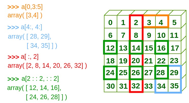
c
array([[[ 1.,  2.,  3.,  4.,  5.],
        [ 6.,  7.,  8.,  9., 10.],
        [11., 12., 13., 14., 15.]],

       [[16., 17., 18., 19., 20.],
        [21., 22., 23., 24., 25.],
        [26., 27., 28., 29., 30.]]])
c[1,1,2]
23.0
e = np.linspace(1,8,8)
e.reshape((2,2,2))
array([[[1., 2.],
        [3., 4.]],

       [[5., 6.],
        [7., 8.]]])
e = np.array([[[1., 2.],[3., 4.]],[[5., 6.],[7., 8.]]])
e
array([[[1., 2.],
        [3., 4.]],

       [[5., 6.],
        [7., 8.]]])
e[0,:,:]*e[1,:,:]
array([[ 5., 12.],
       [21., 32.]])
e[0,:,:]@e[1,:,:]
array([[19., 22.],
       [43., 50.]])
e[0,:,:].dot(e[1,:,:])
array([[19., 22.],
       [43., 50.]])
help(np.linalg.multi_dot)
Help on function multi_dot in module numpy.linalg:

multi_dot(arrays, *, out=None)
    Compute the dot product of two or more arrays in a single function call,
    while automatically selecting the fastest evaluation order.

    `multi_dot` chains `numpy.dot` and uses optimal parenthesization
    of the matrices [1]_ [2]_. Depending on the shapes of the matrices,
    this can speed up the multiplication a lot.

    If the first argument is 1-D it is treated as a row vector.
    If the last argument is 1-D it is treated as a column vector.
    The other arguments must be 2-D.

    Think of `multi_dot` as::

        def multi_dot(arrays): return functools.reduce(np.dot, arrays)


    Parameters
    ----------
    arrays : sequence of array_like
        If the first argument is 1-D it is treated as row vector.
        If the last argument is 1-D it is treated as column vector.
        The other arguments must be 2-D.
    out : ndarray, optional
        Output argument. This must have the exact kind that would be returned
        if it was not used. In particular, it must have the right type, must be
        C-contiguous, and its dtype must be the dtype that would be returned
        for `dot(a, b)`. This is a performance feature. Therefore, if these
        conditions are not met, an exception is raised, instead of attempting
        to be flexible.

        .. versionadded:: 1.19.0

    Returns
    -------
    output : ndarray
        Returns the dot product of the supplied arrays.

    See Also
    --------
    dot : dot multiplication with two arguments.

    References
    ----------

    .. [1] Cormen, "Introduction to Algorithms", Chapter 15.2, p. 370-378
    .. [2] https://en.wikipedia.org/wiki/Matrix_chain_multiplication

    Examples
    --------
    `multi_dot` allows you to write::

    >>> from numpy.linalg import multi_dot
    >>> # Prepare some data
    >>> A = np.random.random((10000, 100))
    >>> B = np.random.random((100, 1000))
    >>> C = np.random.random((1000, 5))
    >>> D = np.random.random((5, 333))
    >>> # the actual dot multiplication
    >>> _ = multi_dot([A, B, C, D])

    instead of::

    >>> _ = np.dot(np.dot(np.dot(A, B), C), D)
    >>> # or
    >>> _ = A.dot(B).dot(C).dot(D)

    Notes
    -----
    The cost for a matrix multiplication can be calculated with the
    following function::

        def cost(A, B):
            return A.shape[0] * A.shape[1] * B.shape[1]

    Assume we have three matrices
    :math:`A_{10x100}, B_{100x5}, C_{5x50}`.

    The costs for the two different parenthesizations are as follows::

        cost((AB)C) = 10*100*5 + 10*5*50   = 5000 + 2500   = 7500
        cost(A(BC)) = 10*100*50 + 100*5*50 = 50000 + 25000 = 75000
np.linalg.multi_dot([e[0,:,:],e[1,:,:]])
array([[19., 22.],
       [43., 50.]])
print(a)
print(c[0,:,:])
r = a.dot(c[0,:,:])
print(r)
print(r.shape)
r.ndim
[ 1.   5.5 10. ]
[[ 1.  2.  3.  4.  5.]
 [ 6.  7.  8.  9. 10.]
 [11. 12. 13. 14. 15.]]
[144.  160.5 177.  193.5 210. ]
(5,)
1
ap = a.reshape((1,3))
print(ap)
ap.shape
rp = ap.dot(c[0,:,:])
print(rp)
print(rp.shape)
rp.ndim
[[ 1.   5.5 10. ]]
[[144.  160.5 177.  193.5 210. ]]
(1, 5)
2
at = a.T
print(at)
at.shape
[ 1. 5.5 10. ]
(3,)
apt = ap.T
print(apt)
apt.shape
[[ 1. ]
 [ 5.5]
 [10. ]]
(3, 1)
print(at)
r = np.ones((3,3)).dot(at)
print(r)
print(r.shape)
r.ndim
[ 1.   5.5 10. ]
[16.5 16.5 16.5]
(3,)
1
print(apt)
r = np.ones((3,3)).dot(apt)
print(r)
print(r.shape)
r.ndim
[[ 1. ]
 [ 5.5]
 [10. ]]
[[16.5]
 [16.5]
 [16.5]]
(3, 1)
2