
ML
Referencia https://planetachatbot.com/como-convertirse-data-scientist-e8f61a83d591
Referencia https://medium.com/@experiencIA18/diferencias-entre-la-inteligencia-artificial-y-el-machine-learning-f0448c503cd4
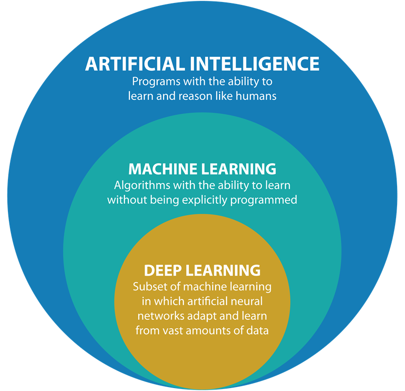
Una definición de ML es la siguiente:
El machine learning es un método de análisis de datos que automatiza la construcción de modelos analíticos. Es una rama de la inteligencia artificial basada en la idea de que los sistemas pueden aprender de datos, identificar patrones y tomar decisiones con mínima intervención humana.
Referencia https://www.sas.com/es_mx/insights/analytics/machine-learning.html
Simplificando bastante esta definición, el ML es un conjunto de algoritmos diseñados para resolver problemas con el uso de datos. Estos problemas se pueden clasificar en tres grandes grupos:
Aprendizaje supervisado. Un modelo se ajusta conociendo las entradas y las salidas asociadas. El objetivo es hacer predicciones en presencia de incertidumbre. Este tipo de aprendizaje se puede dividir en:
Clasificación. Predecir respuestas discretas.
Regresión. Predecir respuestas continuas.
Aprendizaje no supervisado. Encuentra patrones intrínsecos en datos de entrada que no estan asociados a ninguna salida. Este tipo de aprendizaje se puede dividir en
Agrupación. Agrupar los datos de acuerdo a sus características intrínsecas.
Reducción de dimensiones. Reducir el número de características de los datos bajo algún criterio.
Otros algoritmos de aprendizaje. Destacan los algoritmos de Reinformcement Learning. Este tipo de algoritmos determinan qué acciones debe escoger un agente de software en un entorno dado con el fin de maximizar alguna noción de “recompensa” o premio acumulado.

Referencia https://www.sciencedirect.com/science/article/pii/S157401372030071X
Para leer
Machine learning y big data: ¿qué oportunidades ofrecen estas disciplinas para la evaluación de impacto? https://rafneta.github.io/EPSTareas/posts/2020-09-16-machine-learning-y-big-data-qu-oportunidades-nos-ofrece-el-rpido-desarrollo-de-estas-disciplinas-para-la-evaluacin-de-impacto/
Athey, Susan, and Guido W. Imbens. 2019. “Machine Learning Methods That Economists Should Know About.” Annual Review of Economics 11 (1): 685–725. https://doi.org/10.1146/annurev-economics-080217-053433.
Parker, Susan W, and Tom Vogl. 2018. “Do Conditional Cash Transfers Improve Economic Outcomes in the Next Generation? Evidence from Mexico.” Working Paper 24303. Working Paper Series. National Bureau of Economic Research. https://doi.org/10.3386/w24303.
Varian, Hal R. 2014. “Big Data: New Tricks for Econometrics.” Journal of Economic Perspectives 28 (2): 3–28. https://doi.org/10.1257/jep.28.2.3.
Zheng, Eric, Yong Tan, Paulo Goes, Ramnath Chellappa, D.J. Wu, Michael Shaw, Olivia Sheng, and Alok Gupta. n.d. “When Econometrics Meets Machine Learning.” Data and Information Management 1 (2). Berlin: Sciendo: 75–83. https://doi.org/https://doi.org/10.1515/dim-2017-0012.
Extra: Melissa Dell https://twitter.com/MelissaLDell/status/1380173059001307136?s=20
Notas
La forma de insertar ténicas de una área a otra parece subjetiva, es decir, decidir si un algoritmo es propio del ML tiene que ver con la secuencia de cómo se aprendan éstos. Por ejemplo, en el libro The Elements of Statistical Learning Data Mining, Inference, and Prediction (ESoSL), que es considerado un referente para aprender ML, en el capítulo 3: Linear Methods for Regression, se aborda el problema de mínimos cuadrados ordinarios (MCO) de forma similar a como se puede encontrar en libros clásicos de econometría.
Un enunciado simplista para sintetizar el uso de estos métodos en EI, pero que da una perspectiva del objetivo de esta sección, es el siguiente
Para utilizar ML en Economía es necesario describir el problema de Economía como un problema matemático cuya solución pueda implementarse como un algoritmo de ML. Lo cuál no es necesariamente fácil de construir (my feeling)
scikit-learn
scikit-learn. Herramientas simples y eficientes para el análisis de datos, construido sobre Numpy, Scipy y Matplotlib (no es robusto para redes neuronales, para redes neuronales, se puede consultar PyTorch, TensorFlow)
Instalación
conda install -c intel scikit-learn
En la guía de usuario, hay un resumen del problema a resolver, y enlaces a problemas de ejemplo. En el siguiente enlace está la documentación por función
Cargar datos de prueba y datos adquiridos (toy datasets, real datasets).
Para mayor información enlace
Los siguentes códigos son los ejemplos desarrollados en la guía de referencia correspondiente
from sklearn.datasets import load_iris #(para datos de prueba)
data = load_iris()
type(data)
sklearn.utils.Bunch
data
{'data': array([[5.1, 3.5, 1.4, 0.2],
        [4.9, 3. , 1.4, 0.2],
        [4.7, 3.2, 1.3, 0.2],
        [4.6, 3.1, 1.5, 0.2],
        [5. , 3.6, 1.4, 0.2],
        [5.4, 3.9, 1.7, 0.4],
        [4.6, 3.4, 1.4, 0.3],
        [5. , 3.4, 1.5, 0.2],
        [4.4, 2.9, 1.4, 0.2],
        [4.9, 3.1, 1.5, 0.1],
        [5.4, 3.7, 1.5, 0.2],
        [4.8, 3.4, 1.6, 0.2],
        [4.8, 3. , 1.4, 0.1],
        [4.3, 3. , 1.1, 0.1],
        [5.8, 4. , 1.2, 0.2],
        [5.7, 4.4, 1.5, 0.4],
        [5.4, 3.9, 1.3, 0.4],
        [5.1, 3.5, 1.4, 0.3],
        [5.7, 3.8, 1.7, 0.3],
        [5.1, 3.8, 1.5, 0.3],
        [5.4, 3.4, 1.7, 0.2],
        [5.1, 3.7, 1.5, 0.4],
        [4.6, 3.6, 1. , 0.2],
        [5.1, 3.3, 1.7, 0.5],
        [4.8, 3.4, 1.9, 0.2],
        [5. , 3. , 1.6, 0.2],
        [5. , 3.4, 1.6, 0.4],
        [5.2, 3.5, 1.5, 0.2],
        [5.2, 3.4, 1.4, 0.2],
        [4.7, 3.2, 1.6, 0.2],
        [4.8, 3.1, 1.6, 0.2],
        [5.4, 3.4, 1.5, 0.4],
        [5.2, 4.1, 1.5, 0.1],
        [5.5, 4.2, 1.4, 0.2],
        [4.9, 3.1, 1.5, 0.2],
        [5. , 3.2, 1.2, 0.2],
        [5.5, 3.5, 1.3, 0.2],
        [4.9, 3.6, 1.4, 0.1],
        [4.4, 3. , 1.3, 0.2],
        [5.1, 3.4, 1.5, 0.2],
        [5. , 3.5, 1.3, 0.3],
        [4.5, 2.3, 1.3, 0.3],
        [4.4, 3.2, 1.3, 0.2],
        [5. , 3.5, 1.6, 0.6],
        [5.1, 3.8, 1.9, 0.4],
        [4.8, 3. , 1.4, 0.3],
        [5.1, 3.8, 1.6, 0.2],
        [4.6, 3.2, 1.4, 0.2],
        [5.3, 3.7, 1.5, 0.2],
        [5. , 3.3, 1.4, 0.2],
        [7. , 3.2, 4.7, 1.4],
        [6.4, 3.2, 4.5, 1.5],
        [6.9, 3.1, 4.9, 1.5],
        [5.5, 2.3, 4. , 1.3],
        [6.5, 2.8, 4.6, 1.5],
        [5.7, 2.8, 4.5, 1.3],
        [6.3, 3.3, 4.7, 1.6],
        [4.9, 2.4, 3.3, 1. ],
        [6.6, 2.9, 4.6, 1.3],
        [5.2, 2.7, 3.9, 1.4],
        [5. , 2. , 3.5, 1. ],
        [5.9, 3. , 4.2, 1.5],
        [6. , 2.2, 4. , 1. ],
        [6.1, 2.9, 4.7, 1.4],
        [5.6, 2.9, 3.6, 1.3],
        [6.7, 3.1, 4.4, 1.4],
        [5.6, 3. , 4.5, 1.5],
        [5.8, 2.7, 4.1, 1. ],
        [6.2, 2.2, 4.5, 1.5],
        [5.6, 2.5, 3.9, 1.1],
        [5.9, 3.2, 4.8, 1.8],
        [6.1, 2.8, 4. , 1.3],
        [6.3, 2.5, 4.9, 1.5],
        [6.1, 2.8, 4.7, 1.2],
        [6.4, 2.9, 4.3, 1.3],
        [6.6, 3. , 4.4, 1.4],
        [6.8, 2.8, 4.8, 1.4],
        [6.7, 3. , 5. , 1.7],
        [6. , 2.9, 4.5, 1.5],
        [5.7, 2.6, 3.5, 1. ],
        [5.5, 2.4, 3.8, 1.1],
        [5.5, 2.4, 3.7, 1. ],
        [5.8, 2.7, 3.9, 1.2],
        [6. , 2.7, 5.1, 1.6],
        [5.4, 3. , 4.5, 1.5],
        [6. , 3.4, 4.5, 1.6],
        [6.7, 3.1, 4.7, 1.5],
        [6.3, 2.3, 4.4, 1.3],
        [5.6, 3. , 4.1, 1.3],
        [5.5, 2.5, 4. , 1.3],
        [5.5, 2.6, 4.4, 1.2],
        [6.1, 3. , 4.6, 1.4],
        [5.8, 2.6, 4. , 1.2],
        [5. , 2.3, 3.3, 1. ],
        [5.6, 2.7, 4.2, 1.3],
        [5.7, 3. , 4.2, 1.2],
        [5.7, 2.9, 4.2, 1.3],
        [6.2, 2.9, 4.3, 1.3],
        [5.1, 2.5, 3. , 1.1],
        [5.7, 2.8, 4.1, 1.3],
        [6.3, 3.3, 6. , 2.5],
        [5.8, 2.7, 5.1, 1.9],
        [7.1, 3. , 5.9, 2.1],
        [6.3, 2.9, 5.6, 1.8],
        [6.5, 3. , 5.8, 2.2],
        [7.6, 3. , 6.6, 2.1],
        [4.9, 2.5, 4.5, 1.7],
        [7.3, 2.9, 6.3, 1.8],
        [6.7, 2.5, 5.8, 1.8],
        [7.2, 3.6, 6.1, 2.5],
        [6.5, 3.2, 5.1, 2. ],
        [6.4, 2.7, 5.3, 1.9],
        [6.8, 3. , 5.5, 2.1],
        [5.7, 2.5, 5. , 2. ],
        [5.8, 2.8, 5.1, 2.4],
        [6.4, 3.2, 5.3, 2.3],
        [6.5, 3. , 5.5, 1.8],
        [7.7, 3.8, 6.7, 2.2],
        [7.7, 2.6, 6.9, 2.3],
        [6. , 2.2, 5. , 1.5],
        [6.9, 3.2, 5.7, 2.3],
        [5.6, 2.8, 4.9, 2. ],
        [7.7, 2.8, 6.7, 2. ],
        [6.3, 2.7, 4.9, 1.8],
        [6.7, 3.3, 5.7, 2.1],
        [7.2, 3.2, 6. , 1.8],
        [6.2, 2.8, 4.8, 1.8],
        [6.1, 3. , 4.9, 1.8],
        [6.4, 2.8, 5.6, 2.1],
        [7.2, 3. , 5.8, 1.6],
        [7.4, 2.8, 6.1, 1.9],
        [7.9, 3.8, 6.4, 2. ],
        [6.4, 2.8, 5.6, 2.2],
        [6.3, 2.8, 5.1, 1.5],
        [6.1, 2.6, 5.6, 1.4],
        [7.7, 3. , 6.1, 2.3],
        [6.3, 3.4, 5.6, 2.4],
        [6.4, 3.1, 5.5, 1.8],
        [6. , 3. , 4.8, 1.8],
        [6.9, 3.1, 5.4, 2.1],
        [6.7, 3.1, 5.6, 2.4],
        [6.9, 3.1, 5.1, 2.3],
        [5.8, 2.7, 5.1, 1.9],
        [6.8, 3.2, 5.9, 2.3],
        [6.7, 3.3, 5.7, 2.5],
        [6.7, 3. , 5.2, 2.3],
        [6.3, 2.5, 5. , 1.9],
        [6.5, 3. , 5.2, 2. ],
        [6.2, 3.4, 5.4, 2.3],
        [5.9, 3. , 5.1, 1.8]]),
 'target': array([0, 0, 0, 0, 0, 0, 0, 0, 0, 0, 0, 0, 0, 0, 0, 0, 0, 0, 0, 0, 0, 0,
        0, 0, 0, 0, 0, 0, 0, 0, 0, 0, 0, 0, 0, 0, 0, 0, 0, 0, 0, 0, 0, 0,
        0, 0, 0, 0, 0, 0, 1, 1, 1, 1, 1, 1, 1, 1, 1, 1, 1, 1, 1, 1, 1, 1,
        1, 1, 1, 1, 1, 1, 1, 1, 1, 1, 1, 1, 1, 1, 1, 1, 1, 1, 1, 1, 1, 1,
        1, 1, 1, 1, 1, 1, 1, 1, 1, 1, 1, 1, 2, 2, 2, 2, 2, 2, 2, 2, 2, 2,
        2, 2, 2, 2, 2, 2, 2, 2, 2, 2, 2, 2, 2, 2, 2, 2, 2, 2, 2, 2, 2, 2,
        2, 2, 2, 2, 2, 2, 2, 2, 2, 2, 2, 2, 2, 2, 2, 2, 2, 2]),
 'frame': None,
 'target_names': array(['setosa', 'versicolor', 'virginica'], dtype='<U10'),
 'DESCR': '.. _iris_dataset:\n\nIris plants dataset\n--------------------\n\n**Data Set Characteristics:**\n\n    :Number of Instances: 150 (50 in each of three classes)\n    :Number of Attributes: 4 numeric, predictive attributes and the class\n    :Attribute Information:\n        - sepal length in cm\n        - sepal width in cm\n        - petal length in cm\n        - petal width in cm\n        - class:\n                - Iris-Setosa\n                - Iris-Versicolour\n                - Iris-Virginica\n                \n    :Summary Statistics:\n\n    ============== ==== ==== ======= ===== ====================\n                    Min  Max   Mean    SD   Class Correlation\n    ============== ==== ==== ======= ===== ====================\n    sepal length:   4.3  7.9   5.84   0.83    0.7826\n    sepal width:    2.0  4.4   3.05   0.43   -0.4194\n    petal length:   1.0  6.9   3.76   1.76    0.9490  (high!)\n    petal width:    0.1  2.5   1.20   0.76    0.9565  (high!)\n    ============== ==== ==== ======= ===== ====================\n\n    :Missing Attribute Values: None\n    :Class Distribution: 33.3% for each of 3 classes.\n    :Creator: R.A. Fisher\n    :Donor: Michael Marshall (MARSHALL%PLU@io.arc.nasa.gov)\n    :Date: July, 1988\n\nThe famous Iris database, first used by Sir R.A. Fisher. The dataset is taken\nfrom Fisher\'s paper. Note that it\'s the same as in R, but not as in the UCI\nMachine Learning Repository, which has two wrong data points.\n\nThis is perhaps the best known database to be found in the\npattern recognition literature.  Fisher\'s paper is a classic in the field and\nis referenced frequently to this day.  (See Duda & Hart, for example.)  The\ndata set contains 3 classes of 50 instances each, where each class refers to a\ntype of iris plant.  One class is linearly separable from the other 2; the\nlatter are NOT linearly separable from each other.\n\n.. topic:: References\n\n   - Fisher, R.A. "The use of multiple measurements in taxonomic problems"\n     Annual Eugenics, 7, Part II, 179-188 (1936); also in "Contributions to\n     Mathematical Statistics" (John Wiley, NY, 1950).\n   - Duda, R.O., & Hart, P.E. (1973) Pattern Classification and Scene Analysis.\n     (Q327.D83) John Wiley & Sons.  ISBN 0-471-22361-1.  See page 218.\n   - Dasarathy, B.V. (1980) "Nosing Around the Neighborhood: A New System\n     Structure and Classification Rule for Recognition in Partially Exposed\n     Environments".  IEEE Transactions on Pattern Analysis and Machine\n     Intelligence, Vol. PAMI-2, No. 1, 67-71.\n   - Gates, G.W. (1972) "The Reduced Nearest Neighbor Rule".  IEEE Transactions\n     on Information Theory, May 1972, 431-433.\n   - See also: 1988 MLC Proceedings, 54-64.  Cheeseman et al"s AUTOCLASS II\n     conceptual clustering system finds 3 classes in the data.\n   - Many, many more ...',
 'feature_names': ['sepal length (cm)',
  'sepal width (cm)',
  'petal length (cm)',
  'petal width (cm)'],
 'filename': '/Users/rafamtz/opt/anaconda3/lib/python3.8/site-packages/sklearn/datasets/data/iris.csv'}
data.target
array([0, 0, 0, 0, 0, 0, 0, 0, 0, 0, 0, 0, 0, 0, 0, 0, 0, 0, 0, 0, 0, 0,
       0, 0, 0, 0, 0, 0, 0, 0, 0, 0, 0, 0, 0, 0, 0, 0, 0, 0, 0, 0, 0, 0,
       0, 0, 0, 0, 0, 0, 1, 1, 1, 1, 1, 1, 1, 1, 1, 1, 1, 1, 1, 1, 1, 1,
       1, 1, 1, 1, 1, 1, 1, 1, 1, 1, 1, 1, 1, 1, 1, 1, 1, 1, 1, 1, 1, 1,
       1, 1, 1, 1, 1, 1, 1, 1, 1, 1, 1, 1, 2, 2, 2, 2, 2, 2, 2, 2, 2, 2,
       2, 2, 2, 2, 2, 2, 2, 2, 2, 2, 2, 2, 2, 2, 2, 2, 2, 2, 2, 2, 2, 2,
       2, 2, 2, 2, 2, 2, 2, 2, 2, 2, 2, 2, 2, 2, 2, 2, 2, 2])
#https://scikit-learn.org/stable/modules/generated/sklearn.datasets.fetch_california_housing.html#sklearn.datasets.fetch_california_housing
from sklearn.datasets import fetch_california_housing # datos reales

data1 = fetch_california_housing()
data2 = fetch_california_housing(return_X_y=True)
data1
{'data': array([[   8.3252    ,   41.        ,    6.98412698, ...,    2.55555556,
           37.88      , -122.23      ],
        [   8.3014    ,   21.        ,    6.23813708, ...,    2.10984183,
           37.86      , -122.22      ],
        [   7.2574    ,   52.        ,    8.28813559, ...,    2.80225989,
           37.85      , -122.24      ],
        ...,
        [   1.7       ,   17.        ,    5.20554273, ...,    2.3256351 ,
           39.43      , -121.22      ],
        [   1.8672    ,   18.        ,    5.32951289, ...,    2.12320917,
           39.43      , -121.32      ],
        [   2.3886    ,   16.        ,    5.25471698, ...,    2.61698113,
           39.37      , -121.24      ]]),
 'target': array([4.526, 3.585, 3.521, ..., 0.923, 0.847, 0.894]),
 'frame': None,
 'target_names': ['MedHouseVal'],
 'feature_names': ['MedInc',
  'HouseAge',
  'AveRooms',
  'AveBedrms',
  'Population',
  'AveOccup',
  'Latitude',
  'Longitude'],
 'DESCR': '.. _california_housing_dataset:\n\nCalifornia Housing dataset\n--------------------------\n\n**Data Set Characteristics:**\n\n    :Number of Instances: 20640\n\n    :Number of Attributes: 8 numeric, predictive attributes and the target\n\n    :Attribute Information:\n        - MedInc        median income in block\n        - HouseAge      median house age in block\n        - AveRooms      average number of rooms\n        - AveBedrms     average number of bedrooms\n        - Population    block population\n        - AveOccup      average house occupancy\n        - Latitude      house block latitude\n        - Longitude     house block longitude\n\n    :Missing Attribute Values: None\n\nThis dataset was obtained from the StatLib repository.\nhttp://lib.stat.cmu.edu/datasets/\n\nThe target variable is the median house value for California districts.\n\nThis dataset was derived from the 1990 U.S. census, using one row per census\nblock group. A block group is the smallest geographical unit for which the U.S.\nCensus Bureau publishes sample data (a block group typically has a population\nof 600 to 3,000 people).\n\nIt can be downloaded/loaded using the\n:func:`sklearn.datasets.fetch_california_housing` function.\n\n.. topic:: References\n\n    - Pace, R. Kelley and Ronald Barry, Sparse Spatial Autoregressions,\n      Statistics and Probability Letters, 33 (1997) 291-297\n'}
data2
(array([[   8.3252    ,   41.        ,    6.98412698, ...,    2.55555556,
           37.88      , -122.23      ],
        [   8.3014    ,   21.        ,    6.23813708, ...,    2.10984183,
           37.86      , -122.22      ],
        [   7.2574    ,   52.        ,    8.28813559, ...,    2.80225989,
           37.85      , -122.24      ],
        ...,
        [   1.7       ,   17.        ,    5.20554273, ...,    2.3256351 ,
           39.43      , -121.22      ],
        [   1.8672    ,   18.        ,    5.32951289, ...,    2.12320917,
           39.43      , -121.32      ],
        [   2.3886    ,   16.        ,    5.25471698, ...,    2.61698113,
           39.37      , -121.24      ]]),
 array([4.526, 3.585, 3.521, ..., 0.923, 0.847, 0.894]))
X,y = fetch_california_housing(return_X_y=True)
X
array([[   8.3252    ,   41.        ,    6.98412698, ...,    2.55555556,
          37.88      , -122.23      ],
       [   8.3014    ,   21.        ,    6.23813708, ...,    2.10984183,
          37.86      , -122.22      ],
       [   7.2574    ,   52.        ,    8.28813559, ...,    2.80225989,
          37.85      , -122.24      ],
       ...,
       [   1.7       ,   17.        ,    5.20554273, ...,    2.3256351 ,
          39.43      , -121.22      ],
       [   1.8672    ,   18.        ,    5.32951289, ...,    2.12320917,
          39.43      , -121.32      ],
       [   2.3886    ,   16.        ,    5.25471698, ...,    2.61698113,
          39.37      , -121.24      ]])
y
array([4.526, 3.585, 3.521, ..., 0.923, 0.847, 0.894])
Conjunto de entrenamiento y conjunto de prueba
from sklearn.model_selection import train_test_split

X_train, X_test, y_train, y_test = train_test_split(X, y, test_size=.4, random_state=42)