
Contenido
Funciones y métodos
Se pueden realizar cuatro tipos de funciones de acuerdo a sus valors de entrada y salida.
Tipo I. No reciben argumentos de entrada y no tienen valores de salida (no reciben nada y no regresan nada)
Tipo II. No reciben argumentos de entrada y regresa valores de salida (recibe argumento y regresa valores)
Tipo III. Reciben argumentos de entrada y no regresan valores de salida (recibe argumento y no regresa nada)
Tipo IV. Recibe argumentos de entrada regresa y regesa valores de salida (recibe argumento y regresa valores)
El tipo de implemetación depende de las necesidades del problema. Para identificar que tipo de función se esta implementando, basta con observar su implementación.
def funcion_tipoI()
    sentencia_1
    sentencia_2
    ...
    ...
    ...
    sentencia_n
def funcion_tipoII()
    sentencia_1
    sentencia_2
    ...
    ...
    ...
    sentencia_n
    return variable #una o varias veces en el código
def funcion_tipoIII(argumento_1, argumento_2, ..., argumento_n)
    sentencia_1
    sentencia_2
    ...
    ...
    ...
    sentencia_n
def funcion_tipoIV(argumento_1, argumento_2, ..., argumento_n)
    sentencia_1
    sentencia_2
    ...
    ...
    ...
    sentencia_n
    return variable # una o varias veces en el código
Una vez que se realiza la implementación, el uso de la función es con la sigueinte sintaxis:
funcion_tipoI()
funcion_tipoII()
funcion_tipoIII(argumento_1, argumento_2, ..., argumento_n)
funcion_tipoIV(argumento_1, argumento_2, ..., argumento_n)
Los valores que podría calcular una función se pueden utilizar en cualquier parte del código (una vez definida esta) cuando en la implemenación aparezca return en el código de la implementación.
Por ejemplo
Los métodos son funciones asociadas a una clase. Por el momento pensemos a las clases como los tipos de datos. Mostraremos algunos métodos para los tipos de datos string y list
El uso de los métodos tiene la siguiente sintaxis
variable.metodo()
variable.metodo(argumento1,...,argumenton) #cuando el argumento sea necesario
Para los datos tipo string se muestran tres métodos:
Para consultar la descripción de todos los métodos: Métodos para datos tipo string
Para los datos tipo list se muestran un método y dos operaciones:
Para consultar la descripción de todos los métodos: Métodos para datos tipo list
Ejemplo: Módulo Matplotlib
Como es natural de pensar no podemos generar en una computadora conjuntos continuos (pues necesitariamos cantidad infinita de memoria) así que si queremos general gráficas de funciones cuyo dominio es un conjunto continuo, tomamos unas muestras (un subconjunto finito lo suficientemente «bueno») y aplicamos la función, posteriormente con ayuda de la represenación visual emulamos la aplicación de la función a un conjunto infinito. Como principal ayuda para esta parte se puede consultar:
Documentos de matplotlib uno de los módulos escrito en Python para generar gráficas, un módulo extenso.
Galeria de imágenes proporciona el código de las imágenes que se observan
Documentos de matplotlib.pyplot submódulo de matplotlib para generar gráficas, donde se tiene una sintaxys tipo MATLAB (esto es bueno si sabes MATLAB)
Documento de plot una de las descripciones que se puede encontrar en la página anterior
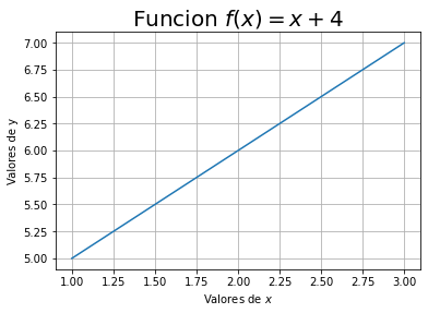
import matplotlib.pyplot as plt
#Principio básico del plot
x=[1,2,3]
y=[5,6,7]
plt.plot(x,y)
plt.grid()
plt.title(r'Funcion $f(x)=x+4$', fontsize=20)
plt.xlabel('Valores de $x$')
plt.ylabel('Valores de y')
plt.show()
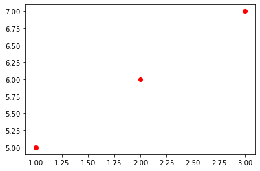
plt.plot(x,y,'ro')
plt.show()
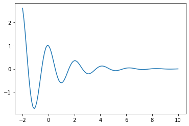
Generar la gráfica de la siguiente función
def puntos_x(a,b, h = 1):
    x = list()
    for i in range(round((b - a) / h) + 1):
        x = x + [a + i * h]
    return x

import math


li = -2
ls = 10
paso = 0.1


valores_x = puntos_x(li, ls, paso)

numero_puntos = len(valores_x)

f = list()

for i in range(numero_puntos):
    f.append(math.exp(-0.5 * valores_x[i]) * math.cos(3 * valores_x[i]))

#print(f)

plt.plot(valores_x,f)
plt.show()
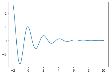
Se complica la generación de listas y sobre todo manipular y aplicar funciones a cada uno de los elementos (uso de ciclos). El módulo numpy nos porporciona un tipo de dato que se llama array el cual junto con las funciones matemáticas de numpy permite un uso directo de las evaluaciones de funciones a todos los elementos del array. El módulo es extenso y contiene submódulos al igual que matplotlib con diferentes herramientas matemáticas. La ayuda se puede encontrar en el siguiente enlace
-Documentos de numpy Manual del módulo numpy.
import numpy as np

x = np.linspace(-2, 10, 300)
y = np.exp(-0.5 * x) * np.cos(3 * x)
plt.plot(x, y)
plt.show()
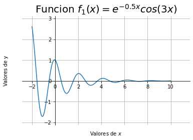
x=np.linspace(-2, 10, 300)
y=np.exp(-0.5 * x) * np.cos(3 * x)
plt.plot(x, y)
plt.grid()
plt.title('Funcion $f_1(x)=e^{-0.5x}cos(3x)$', fontsize = 20)
plt.xlabel('Valores de $x$')
plt.ylabel('Valores de y')
ax = plt.gca()
ax.xaxis.set_label_coords(0.5, -0.05)
ax.yaxis.set_label_coords(-0.08, 0.5)
ax.spines['right'].set_color('none')
ax.spines['top'].set_color('none')
ax.xaxis.set_ticks_position('bottom')
ax.spines['bottom'].set_position(('data', 0))
ax.yaxis.set_ticks_position('left')
ax.spines['left'].set_position(('data', 0))
xlim=ax.get_xlim()
ylim=ax.get_ylim()
ax.set_xlim(min(xlim[0] * (0.9), xlim[0] * (1.1)), max(xlim[1] * 1.1, xlim[1] * 0.9))
ax.set_ylim(min(ylim[0] * (0.9), ylim[0] * (1.1)), max(ylim[1] * 1.1, ylim[1] * 0.9))
plt.show()
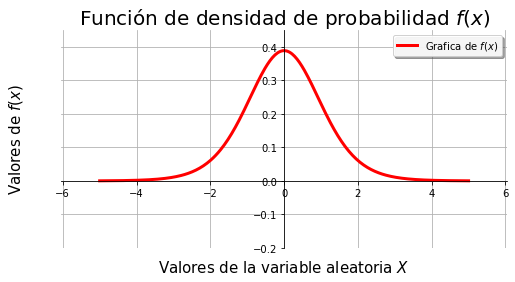
Es un poco tardado dar un formato deseado a las gráficas, entonces el uso de funciones se vuelve fundamental. Los siguiente códigos grafican funciones, pensando que se quieren gráficar funciones de densidad de probablidlidad y de distribución acumulada.
def gfdvac(Intervalo,f,titulo='Funcion de densidad de probabilidad $f(x)$', guardar = False):
    fig=plt.figure(figsize=(8,4))#
    ax=plt.axes()
    x=np.linspace(Intervalo[0],Intervalo[1],300)
    y=f(x)
    ax.plot(x,y,c = 'r',lw = 3,label = r'Grafica de $f(x)$')
    ax.grid()
    ax.set_xlabel('Valores de la variable aleatoria $X$', fontsize = 15)
    ax.set_ylabel('Valores de $f(x)$', fontsize = 15)
    ax.set_title('Función de densidad de probabilidad $f(x)$',fontsize = 20)
    leg = plt.legend(loc='best', shadow = True, fancybox = True)
    leg.get_frame().set_alpha(0.9)
    ax.xaxis.set_label_coords(0.5, -0.05)
    ax.yaxis.set_label_coords(-0.08, 0.5)
    ax.spines['right'].set_color('none')
    ax.spines['top'].set_color('none')
    ax.xaxis.set_ticks_position('bottom')
    ax.spines['bottom'].set_position(('data',0))
    ax.yaxis.set_ticks_position('left')
    ax.spines['left'].set_position(('data',0))
    xlim=ax.get_xlim()
    ylim=ax.get_ylim()
    ax.set_xlim(min(xlim[0] * (0.9), xlim[0] * (1.1)), max(xlim[1] * 1.1, xlim[1] * 0.9))
    ax.set_ylim(-0.2,max(ylim[1] * 1.1, ylim[1] * 0.9))
    if guardar:
        plt.savefig("fvac.png")# Se puede guardar solo en el formato deseado
        plt.savefig("fvac.pdf")#
        #plt.savefig("fvac.jpg")#
    plt.show()
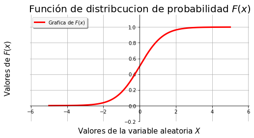
def gFdvac(Intervalo,F,titulo='Función de distribucion de probabilidad $F(x)$',\
          guardar=False):
    fig=plt.figure(figsize=(8,4))#
    ax=plt.axes()
    x=np.linspace(Intervalo[0],Intervalo[1],300)
    y=F(x)
    ax.plot(x,y,c='r',lw=3,label=r'Grafica de $F(x)$')
    ax.grid()
    ax.set_xlabel('Valores de la variable aleatoria $X$',fontsize=15)
    ax.set_ylabel('Valores de $F(x)$',fontsize=15)
    ax.set_title('Función de distribcucion de probabilidad $F(x)$',fontsize=20)
    leg = plt.legend(loc='best', shadow=True, fancybox=True)
    leg.get_frame().set_alpha(0.9)
    ax.xaxis.set_label_coords(0.5, -0.05)
    ax.yaxis.set_label_coords(-0.08,0.5)
    ax.spines['right'].set_color('none')
    ax.spines['top'].set_color('none')
    ax.xaxis.set_ticks_position('bottom')
    ax.spines['bottom'].set_position(('data',0))
    ax.yaxis.set_ticks_position('left')
    ax.spines['left'].set_position(('data',0))
    xlim=ax.get_xlim()
    ylim=ax.get_ylim()
    ax.set_xlim(min(xlim[0]*(0.9),xlim[0]*(1.1)),max(xlim[1]*1.1,xlim[1]*0.9))
    ax.set_ylim(-0.2,max(ylim[1]*1.1,ylim[1]*0.9))
    if guardar:
        plt.savefig("Fvac.png")# Se puede guardar solo en el formato deseado
        plt.savefig("Fvac.pdf")#
        #plt.savefig("Fvac.jpg")#
    plt.show()
Ejemplo: Módulo para estadística stats
stats es un submódulo de scipy para estadística
-Documento Scipy. Módulo para computación cientifica compatible con Numpy y Matplotlib, entre otros
-scipy módulo stats. Información de stats
Variables aleatorias continuas
pdf(x) (Probability Density Function) Función de densidad \(f(x)=F'(x)\)
cdf(x) (Cumulative Distribution Function) Funcion de distribución \(F(x)\)
ppf(x) (Percent Point Function) Función inversa a cdf(x) \(G(q)=F^{-1}(q)\)
from scipy import stats # importando scipy.stats
# Ya se ha importando scipy.stats
# loc=0, scale=1, df=n
vct = stats.t(df=10)
f = vct.pdf
F = vct.cdf
gfdvac((-5,5),f, guardar = True) #de acuerdo a como se programo
gFdvac((-5,5),F)
#gFdfvac((-5,5),f)
print(vct.mean())
print(vct.median())
print(vct.var())
print(vct.std())
0.0
6.80574793290978e-17
1.25
1.118033988749895
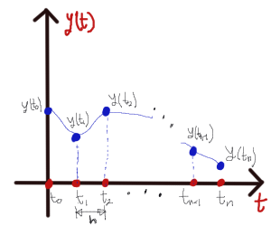
Ejemplo: Ecuación diferencial
Se pueden realizar aproximaciones numéricas a ecuaciones diferenciales. El siguiente es una motivación del método de Euler (la deducción es por medio de series de Taylor)
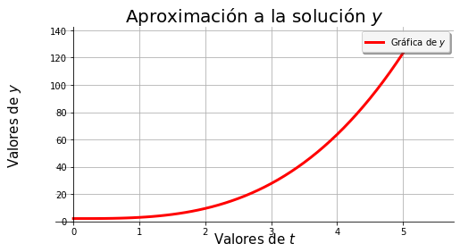
Problema 1
Encontrar una aproximación numérica a
en el intervalo \([0,5]\) con paso \(h=0.1\)
def f1(y,t):
    return 3 * t ** 2
def euler(f, a, b, y0 = 0, paso = 0.1, sol = None):

    vect = puntos_x(a, b, paso)

    y = [y0]

    for t in vect[0:-1]:
        y.append(y[-1]+ f(y[-1],t)*paso)
    print(vect, y)
euler(f1, 0, 5, 2)
[0.0, 0.1, 0.2, 0.30000000000000004, 0.4, 0.5, 0.6000000000000001, 0.7000000000000001, 0.8, 0.9, 1.0, 1.1, 1.2000000000000002, 1.3, 1.4000000000000001, 1.5, 1.6, 1.7000000000000002, 1.8, 1.9000000000000001, 2.0, 2.1, 2.2, 2.3000000000000003, 2.4000000000000004, 2.5, 2.6, 2.7, 2.8000000000000003, 2.9000000000000004, 3.0, 3.1, 3.2, 3.3000000000000003, 3.4000000000000004, 3.5, 3.6, 3.7, 3.8000000000000003, 3.9000000000000004, 4.0, 4.1000000000000005, 4.2, 4.3, 4.4, 4.5, 4.6000000000000005, 4.7, 4.800000000000001, 4.9, 5.0] [2, 2.0, 2.003, 2.015, 2.0420000000000003, 2.0900000000000003, 2.1650000000000005, 2.2730000000000006, 2.420000000000001, 2.612000000000001, 2.855000000000001, 3.155000000000001, 3.518000000000001, 3.950000000000001, 4.457000000000001, 5.045000000000001, 5.720000000000001, 6.488000000000001, 7.355000000000001, 8.327000000000002, 9.410000000000002, 10.610000000000003, 11.933000000000003, 13.385000000000003, 14.972000000000003, 16.700000000000003, 18.575000000000003, 20.603, 22.790000000000003, 25.142000000000003, 27.665000000000003, 30.365000000000002, 33.248000000000005, 36.32000000000001, 39.58700000000001, 43.055000000000014, 46.73000000000001, 50.61800000000001, 54.72500000000001, 59.05700000000001, 63.62000000000001, 68.42000000000002, 73.46300000000002, 78.75500000000002, 84.30200000000002, 90.11000000000003, 96.18500000000003, 102.53300000000003, 109.16000000000003, 116.07200000000003, 123.27500000000003]
def grafica(vect, y, solucion = None, titulo='Aproximación a la solución', guardar=False):
    fig=plt.figure(figsize=(8,4))#
    ax=plt.axes()
    ax.plot(vect, y, c = 'r', lw = 3, label = 'Gráfica de $y$')
    ax.grid()
    ax.set_xlabel('Valores de $t$', fontsize = 15)
    ax.set_ylabel('Valores de $y$', fontsize = 15)
    ax.set_title('Aproximación a la solución $y$',fontsize = 20)
    leg = plt.legend(loc = 'best', shadow = True, fancybox = True)
    leg.get_frame().set_alpha(0.9)
    ax.xaxis.set_label_coords(0.5, -0.05)
    ax.yaxis.set_label_coords(-0.08,0.5)
    ax.spines['right'].set_color('none')
    ax.spines['top'].set_color('none')
    ax.xaxis.set_ticks_position('bottom')
    ax.spines['bottom'].set_position(('data',0))
    ax.yaxis.set_ticks_position('left')
    ax.spines['left'].set_position(('data',0))
    xlim=ax.get_xlim()
    ylim=ax.get_ylim()
    ax.set_xlim(min(xlim[0] * (0.9), xlim[0] * (1.1)), max(xlim[1] * 1.1, xlim[1] * 0.9))
    ax.set_ylim(-0.2, max(ylim[1] * 1.1, ylim[1] * 0.9))

    if solucion != None:
        plt.plot(vect,solucion)


    if guardar:
        plt.savefig("Fvac.png")# Se puede guardar solo en el formato deseado
        plt.savefig("Fvac.pdf")#
        #plt.savefig("Fvac.jpg")#
    plt.show()
def euler(f, a, b, y0 = 0, paso = 0.1, sol = None):

    vect = puntos_x(a, b, paso)

    y = [y0]

    for t in vect[0:-1]:
        y.append(y[-1]+ f(y[-1],t)*paso)
    grafica(vect, y, solucion = sol)
euler(f1, 0, 5, 2)
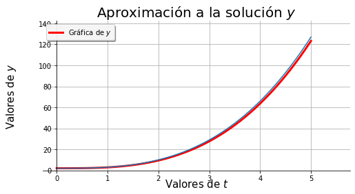
# solución analitica


def f1sol(t):
    return  t ** 3 + 2


def euler(f, a, b, y0 = 0, paso = 0.1, sol = None):

    vect = puntos_x(a, b, paso)

    y = [y0]

    for t in vect[0:-1]:
        y.append(y[-1]+ f(y[-1],t)*paso)

    if sol != None:
        ana = []
        for t in vect:
            ana.append(sol(t))
        grafica(vect, y, solucion = ana)
    else:
        grafica(vect, y)
euler(f1, 0, 5, 2, sol = f1sol)
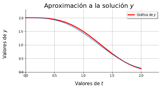
Problema 2
Encontrar una aproximación numérica a
en el intervalo \([0,2]\) con paso \(h=0.1\)
def f2(y,t):
    return -t**2*y

def f2sol(t):
    return 2*math.exp(-t**3/3)

euler(f2, 0, 2, 2, 0.1, f2sol)
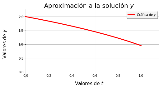
Problema 3
Encontrar una aproximación numérica a
en el intervalo \([0,1]\) con paso \(h=0.1\)
def f3(y,x):
    return (2*x+3*y+1)/(3*x-2*y-5)


euler(f3, 0, 1, 2, 0.1)

Algunas ecuaciones no tendrán una aproximación numérica que se implemente de manera sencilla. Por lo que se pude recurrir funciones ya destiandas para resolver estos problemas, incluso con ello, algunas funciones son lo bastante sofisticadas que establecer algunos argumentos de entrada es complicado (de no conocerse la teoría del método). Por ejemplo revise la documentación de solve_ivp del submódulo integrate del módulo scipy, que es una función para resolver problemas de valor inicial.
from scipy.integrate import solve_ivp


def f3(x,y):
    return (2*x+3*y+1)/(3*x-2*y-5)

sol = solve_ivp(f3, [0,1], [2], max_step = 0.1)

print(sol)
type(sol)
  message: 'The solver successfully reached the end of the integration interval.'
     nfev: 68
     njev: 0
      nlu: 0
      sol: None
   status: 0
  success: True
        t: array([0. , 0.1, 0.2, 0.3, 0.4, 0.5, 0.6, 0.7, 0.8, 0.9, 1. , 1. ])
 t_events: None
        y: array([[2.        , 1.92038615, 1.83686967, 1.74905429, 1.65645985,
        1.55849435, 1.45441243, 1.34325145, 1.22372797, 1.09405967,
        0.9516335 , 0.9516335 ]])
 y_events: None
scipy.integrate._ivp.ivp.OdeResult
#def grafica(vect, y, solucion = None, titulo='Aproximación a la solución', guardar=False):

grafica(sol.t, list(sol.y[0]))
Ejemplos: Problemas generales
Problema
The number 3797 has an interesting property. Being prime itself, it is possible to continuously remove digits from left to right, and remain prime at each stage: 3797, 797, 97, and 7. Similarly we can work from right to left: 3797, 379, 37, and 3.
Find the sum of the only eleven primes that are both truncatable from left to right and right to left.
NOTE: 2, 3, 5, and 7 are not considered to be truncatable primes
No se implementará la solución, porque es un problema propuesto en un sitio especifico
Se impleemntará un bosquejo de una solución, no necesariamente eficiente (con eficiente nos referimos a qeu tarde poco)
Problemas de este tipo se encuentran en Proyect Euler
# Utilizamos la congetura de Agoh–Giuga para saber si un número es primo

def primo(p):

    if p == 1:
        return False
    elif (math.factorial(p - 1) + 1) % p == 0:
        return True
    else:
        return False


# Buscamos de izquierda a derecha para saber si es primo truncable

def primo_id(p):
    ps = str(p)
    for i in range(len(ps)):
        ps_trun = ps[i:]
        # print(i,ps_trun)
        ps_trun_i = int(ps_trun)
        if not primo(ps_trun_i):
            return False
    return True


# Dada una secuencia nos quedamos con los primos truncables

def secuencia(lista):

    truncables = []

    for i in lista:
        if primo_id(i):
            truncables.append(i)
    return truncables


def mensaje():

    print("Hola, este programa implementa una solución parcial del problema 20 de\n\
    Proyect Euler, dada una lista de numeros regresa la suma\n \
    de los elementos que sean primos trucables de izquierda a derecha\n")
mensaje()
L = range(11,500)
p_trun = secuencia(L)
print("la lista es: ",p_trun,'\n')
print("la suma es:" + str(sum(p_trun)))
Hola, este programa implementa una solución parcial del problema 20 de
    Proyect Euler, dada una lista de numeros regresa la suma
     de los elementos que sean primos trucables de izquierda a derecha

la lista es:  [13, 17, 23, 37, 43, 47, 53, 67, 73, 83, 97, 103, 107, 113, 137, 167, 173, 197, 223, 283, 307, 313, 317, 337, 347, 353, 367, 373, 383, 397, 443, 467]

la suma es:6460
primo_id(3797)
True
a = 'hola'
a[3:3]
''
Apéndice
Ayuda y docstring
help(sum)
Help on built-in function sum in module builtins:

sum(iterable, /, start=0)
    Return the sum of a 'start' value (default: 0) plus an iterable of numbers

    When the iterable is empty, return the start value.
    This function is intended specifically for use with numeric values and may
    reject non-numeric types.
?sum
help(str.find)
Help on method_descriptor:

find(...)
    S.find(sub[, start[, end]]) -> int

    Return the lowest index in S where substring sub is found,
    such that sub is contained within S[start:end].  Optional
    arguments start and end are interpreted as in slice notation.

    Return -1 on failure.
dir(str)
['__add__',
 '__class__',
 '__contains__',
 '__delattr__',
 '__dir__',
 '__doc__',
 '__eq__',
 '__format__',
 '__ge__',
 '__getattribute__',
 '__getitem__',
 '__getnewargs__',
 '__gt__',
 '__hash__',
 '__init__',
 '__init_subclass__',
 '__iter__',
 '__le__',
 '__len__',
 '__lt__',
 '__mod__',
 '__mul__',
 '__ne__',
 '__new__',
 '__reduce__',
 '__reduce_ex__',
 '__repr__',
 '__rmod__',
 '__rmul__',
 '__setattr__',
 '__sizeof__',
 '__str__',
 '__subclasshook__',
 'capitalize',
 'casefold',
 'center',
 'count',
 'encode',
 'endswith',
 'expandtabs',
 'find',
 'format',
 'format_map',
 'index',
 'isalnum',
 'isalpha',
 'isascii',
 'isdecimal',
 'isdigit',
 'isidentifier',
 'islower',
 'isnumeric',
 'isprintable',
 'isspace',
 'istitle',
 'isupper',
 'join',
 'ljust',
 'lower',
 'lstrip',
 'maketrans',
 'partition',
 'replace',
 'rfind',
 'rindex',
 'rjust',
 'rpartition',
 'rsplit',
 'rstrip',
 'split',
 'splitlines',
 'startswith',
 'strip',
 'swapcase',
 'title',
 'translate',
 'upper',
 'zfill']
help(dir)
Help on built-in function dir in module builtins:

dir(...)
    dir([object]) -> list of strings

    If called without an argument, return the names in the current scope.
    Else, return an alphabetized list of names comprising (some of) the attributes
    of the given object, and of attributes reachable from it.
    If the object supplies a method named __dir__, it will be used; otherwise
    the default dir() logic is used and returns:
      for a module object: the module's attributes.
      for a class object:  its attributes, and recursively the attributes
        of its bases.
      for any other object: its attributes, its class's attributes, and
        recursively the attributes of its class's base classes.
dir()
['F',
 'In',
 'L',
 'Out',
 '_',
 '_19',
 '_23',
 '_24',
 '_28',
 '__',
 '___',
 '__builtin__',
 '__builtins__',
 '__doc__',
 '__loader__',
 '__name__',
 '__package__',
 '__spec__',
 '_dh',
 '_i',
 '_i1',
 '_i10',
 '_i11',
 '_i12',
 '_i13',
 '_i14',
 '_i15',
 '_i16',
 '_i17',
 '_i18',
 '_i19',
 '_i2',
 '_i20',
 '_i21',
 '_i22',
 '_i23',
 '_i24',
 '_i25',
 '_i26',
 '_i27',
 '_i28',
 '_i29',
 '_i3',
 '_i30',
 '_i4',
 '_i5',
 '_i6',
 '_i7',
 '_i8',
 '_i9',
 '_ih',
 '_ii',
 '_iii',
 '_oh',
 'a',
 'ax',
 'euler',
 'exit',
 'f',
 'f1',
 'f1sol',
 'f2',
 'f2sol',
 'f3',
 'gFdvac',
 'get_ipython',
 'gfdvac',
 'grafica',
 'i',
 'li',
 'ls',
 'math',
 'mensaje',
 'np',
 'numero_puntos',
 'p_trun',
 'paso',
 'plt',
 'primo',
 'primo_id',
 'puntos_x',
 'quit',
 'secuencia',
 'sol',
 'solve_ivp',
 'stats',
 'valores_x',
 'vct',
 'x',
 'xlim',
 'y',
 'ylim']
Asigmación Múltiple
tipo, x, y, z, variable = 'Cadena', -1, 2.6, 10, True
print(tipo, type(tipo))
print(x, type(x))
print(y, type(y))
print(z, type(z))
print(variable, type(variable))
Cadena <class 'str'>
-1 <class 'int'>
2.6 <class 'float'>
10 <class 'int'>
True <class 'bool'>